Large-scale cortical travelling waves predict localized future cortical signals

Abstract

Predicting future brain signal is highly sought-after, yet difficult to achieve. To predict the future phase of cortical activity at localized ECoG and MEG recording sites, we exploit its predominant, large-scale, spatiotemporal dynamics. The dynamics are extracted from the brain signal through Fourier analysis and principal components analysis (PCA) only, and cast in a data model that predicts future signal at each site and frequency of interest. The dominant eigenvectors of the PCA that map the large-scale patterns of past cortical phase to future ones take the form of smoothly propagating waves over the entire measurement array. In ECoG data from 3 subjects and MEG data from 20 subjects collected during a self-initiated motor task, mean phase prediction errors were as low as 0.5 radians at local sites, surpassing state-of-the-art methods of within-time-series or event-related models. Prediction accuracy was highest in delta to beta bands, depending on the subject, was more accurate during episodes of high global power, but was not strongly dependent on the time-course of the task. Prediction results did not require past data from the to-be-predicted site. Rather, best accuracy depended on the availability in the model of long wavelength information. The utility of large-scale, low spatial frequency traveling waves in predicting future phase activity at local sites allows estimation of the error introduced by failing to account for irreducible trajectories in the activity dynamics.

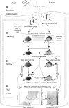
Fig 1

Schematic of analysis workflow A. Temporal relationships between predictor and predicted signal. The raw time-series is first analyzed using short-time-window Morlet wavelets to estimate the phase. The predictor and predicted phase are estimated from non-overlapping portions of the raw time-series. Since each phase estimate requires a window of the raw time-series (brackets), and this window is larger at low frequencies, this means the minimum temporal delay (milliseconds) between past and future phase estimates increases with decreasing frequency. The temporal delay was one cycle at the frequency of interest for the ECoG analysis, and two cycles for the MEG. B. Training stage. Principal components analysis (PCA) is used to empirically derive the spatio-temporal Fourier components. For a single subject, and for a single frequency, all the pairs past-future phase vectors available over all training trials were entered as cases into the PCA. The eigenvectors produced by the PCA were used as basis functions in the subsequent modelling. Each basis function was comprised of a past and future representation of the signal, by virtue of the structure of the paired input vectors. The site to be predicted was also chosen during the training stage, by finding the best predicted site from the future part of the model. For some analyzes, the training stage was performed again from scratch, save with the to-be-predicted site now omitted from the past part of the training vector. The most anterior site, most posterior, most superior and left-most site, are indicated by the letters A, P, S and L, respectively. C. Testing stage. A new past sample of phase (over all measurement sites, or possibly excluding the to-be-predicted site) from the test data set is used to estimate a set of model weights via regression onto the past part of the basis functions. These weights are then used to create a model representation of the future activity. The model phase at the to-be-predicted site is then compared to the actual phase that occurs at that site, forward in time. D. Fits of the past model and errors at the to-be-predicted future site. Left panel shows the fit of the past model to the past samples, averaged at each sample-within-trial; over trials (see Methods). The trial-averaged prediction error, for each sample, at the to-be-predicted future site is shown in the right panel (see methods). The critical feature to note is that each past sample is offset from its paired future sample by a delay that decreases with frequency, due to the requirement that phase be estimated from non-overlapping regions of the raw signal. Four equally spaced time-samples are indicated by ‘bins’ within the plot of past model fits, and their corresponding paired four future samples are likewise indicated within the plot of prediction errors. The paired samples have a corresponding representation in A, as the middle of the three frequencies shown. The relationship between frequency in the output plots (D) and the phase estimation windows for the raw time-series (A, brackets) is indicated by fine dashed lines. The second of the four paired past/future samples, at the middle frequency shown in A, is indicated by its position in the two output plots (D) via the half-circles brackets joined by bold dotted lines.

Fig 2. Example predictive models and prediction errors.

The inset figure has two panels. The first panel gives the relative size and spacing of the measurement arrays for two subjects. The three axes are ‘AP’: anterior-posterior; ‘IS’: inferior-superior; ‘LR’: left-right. A typical phase gradient is shown in colour from the scalar values of phase. The second panel shows the distributions of estimated spatial frequency of the measured phase, over all trials and samples for the subject. The distribution of estimated spatial frequency of phase gradients (see Methods) is shown for all samples in grey. The figure is composed by overlay of samples drawn from the top third of prediction accuracy (red), middle third (green), and lower third (blue). Since selection by prediction accuracy does not alter the distribution, the combined plot is mostly grey. The main figure is broken into five panels. The first four panels show the past phase (as a head map and on the complex plane), the past model phase, the model prediction of the future phase, the actual future phase. For the past phase and future phase panels, head maps are shown in the centre of the panel, with unit circle of phase surrounding. The colours are used to represent phase in both head and circle, and phase is reiterated as angular position on the unit phase circle. For the past model and model prediction, the model output is shown on the complex plane in the centre of the panel. The argument of the model phase i.e. the angle, is shown in colours here and on the model head map (top left of these two panels). The site to be predicted is indicated with a black circle in both the model prediction panel and the future phase panel. These two example predictions are built using only the first eigenvector from the PCA, and therefore the second and third panels illustrate that eigenvector. Upper row: Subject MEG 6, centre frequency 2.0Hz, to-be-predicted site left out of past model. The letters ‘A’, ‘P’, ‘I’, ‘S’, ‘L’, ‘R’ indicate the position of the anterior-most (posterior-most etc.) recording site on either the head map or the unit circle of phase. The site to be predicted is missing from the past model representation, on the bottom row of sensors, just to the right of the ‘L’ sensor. This snapshot is taken during the third trial, at 364ms. See S1 Video, for the first three trials of this subject. Lower row: Subject ECoG 1, centre frequency 6.7Hz. The letters ‘A1’, ‘A8’, ‘H1’, ‘H8’ indicate the labels and positions of the corner recording sites of the ECoG array. The site to be predicted is missing from the past model representation, in position ‘B6’ i.e. one column in from the left, three rows down. This snapshot is taken during the first trial, at -250ms. See S2 Video, for the first three trials of this subject. In the fifth panel (lower right of figure), the mean prediction error is shown with a black arrow for Subject MEG 6 at 354ms, 2.0Hz (upper) and Subject ECoG 1 at -250ms, 6.7Hz (lower). The prediction errors are for a specific site, chosen as the to-be-predicted site during the model construction phase. The phase locking value (PLV) is the real part (i.e. the length of this arrow along the x-axis), here, 0.58 and 0.64 respectively. The prediction errors for each individual trial are also shown with coloured crosses, hot colours are trials with high mean log power, cold colours with low. The prediction error for the trial shown in Fig 1 is indicated with a black cross.

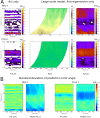
Fig 3. Temporal Fourier model and large-scale model results for two subjects over all samples and frequencies, single eigenvector only.

A. The left plots show the PLV_error for the model that used only the temporal information at the site to be predicted. All values are from the test data set, for the same site analyzed in the middle and right panels. Middle plots show the fit of the past phase data to past model, Ω, the right plot shows the PLV_error for the best predicted site, chosen during model construction. All values are from the test data set. Both Ω and PLV_error extend over 1 second of data, and each sample in the past plot corresponds to the prediction error of the same sample in the future plot. The past plot samples are offset backwards time by either one (ECoG) or two (MEG) cycles at the frequency of interest, indicated by the curved boundaries. Blank regions within the future plot indicate PLV_error less than zero. B. The same future prediction errors as (A), expressed as the standard deviation of the error angle. Colour scale is in radians. The time-only Fourier model results are shown in the first and third panels, the large-scale spatio-temporal Fourier model results are shown in the second and fourth panels.

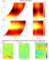
Fig 4. Mean log power and its relationship to model prediction error.

Upper plots show MLP for the same two subjects in previous figures. MLP is normalized over the frequency range by subtracting a linear ramp as a function of frequency, so that event-related changes are emphasized rather than the 1/f power gradient. Conventions are otherwise the same as Fig 3. Lower plots show the time by frequency matrix of correlations between past MLP and prediction error. The real part of the trial-wise error vector (plots one and two) was generally correlated positively with the trial-wise past MLP. The PLV_error (plot three) was generally positively correlated with subject-wise past MLP.

Fig 5. Event-related model results.

PLV_error for the event-related model, the best predicted site at each frequency, chosen during model construction. Values are from the test data set for one MEG subject and one ECoG subject. The figure shows the prediction results for single hand motor activity (left, right or contralateral, ipsilateral) or for modelling results where the two trial-types were combined in the same analysis (both).

Fig 6. Trials selected by past MLP, model using single eigenvector, to-be-predicted site left out of past model.

Only test trials where the past MLP was in the top quartile are included in this plot. Conventions are otherwise the same as for Fig 3.

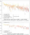
Fig 7. Mean error and SEM at best frequency and time for models with different wave-number and other model parameterizations.

The results are shown for a quarter of the trials, those with the highest past MLP. Upper: results for the event-related model and large-scale TW model (unrotated PCA), across all subjects. Each subject’s PLV_error, at the best time and frequency for that subject, are shown using circles. The event-related model and the models using only the first eigenvector are shown with smallest circles, and other configurations of eigenvectors are shown with successively larger circles, as indicated. Standard error of mean for the real part of the prediction error vector is shown in shaded regions (each subject’s n given in Table 1. The ‘μ’ column indicates the subject-wise mean of PLV_error, and the subject-wise SEM of the PLV_error (n=23). MEG subjects are prefixed by ‘M’, ECoG subjects prefixed by ‘E’. Lower: results using the first eigenvector only, across all subjects. The plot compares unrotated PCA (smallest circles) with rotated PCA and the model with the to-be-predicted site removed, as indicated by the larger circles. Conventions are otherwise the same as for the upper figure.

References

1. Zrenner C, Belardinelli P, Müller-Dahlhaus F, Ziemann U. Closed-Loop Neuroscience and Non-Invasive Brain Stimulation: A Tale of Two Loops. Front Cell Neurosci. 2016;10 10.3389/fncel.2016.00092 - DOI - PMC - PubMed
1. Zhang H, Watrous AJ, Patel A, Jacobs J. Theta and Alpha Oscillations Are Traveling Waves in the Human Neocortex. Neuron. 2018;98: 1269–1281.e4. 10.1016/j.neuron.2018.05.019 - DOI - PMC - PubMed
1. Alexander DM, Jurica P, Trengove C, Nikolaev AR, Gepshtein S, Zvyagintsev M, et al. Traveling waves and trial averaging: the nature of single-trial and averaged brain responses in large-scale cortical signals. NeuroImage. 2013;73: 95–112. 10.1016/j.neuroimage.2013.01.016 - DOI - PubMed
1. Bahramisharif A, Gerven MAJ van, Aarnoutse EJ, Mercier MR, Schwartz TH, Foxe JJ, et al. Propagating Neocortical Gamma Bursts Are Coordinated by Traveling Alpha Waves. J Neurosci. 2013;33: 18849–18854. 10.1523/JNEUROSCI.2455-13.2013 - DOI - PMC - PubMed
1. Ray S, Maunsell JHR. Network Rhythms Influence the Relationship between Spike-Triggered Local Field Potential and Functional Connectivity. J Neurosci. 2011;31: 12674–12682. 10.1523/JNEUROSCI.1856-11.2011 - DOI - PMC - PubMed
Publication types