Gene Expression Changes and Community Turnover Differentially Shape the Global Ocean Metatranscriptome

Abstract

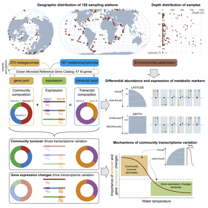
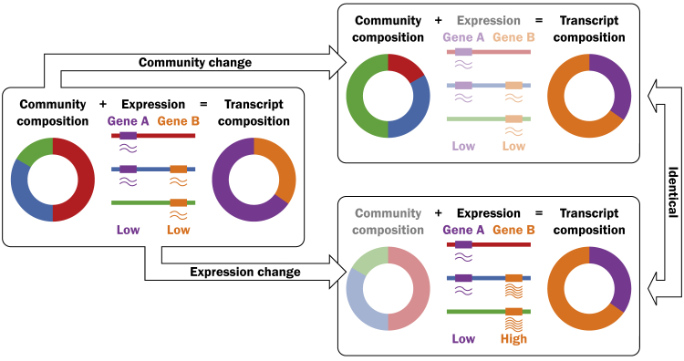
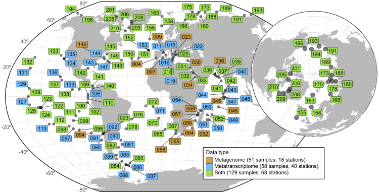
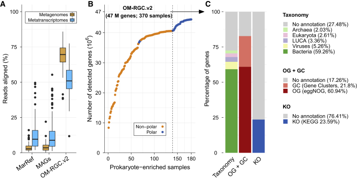
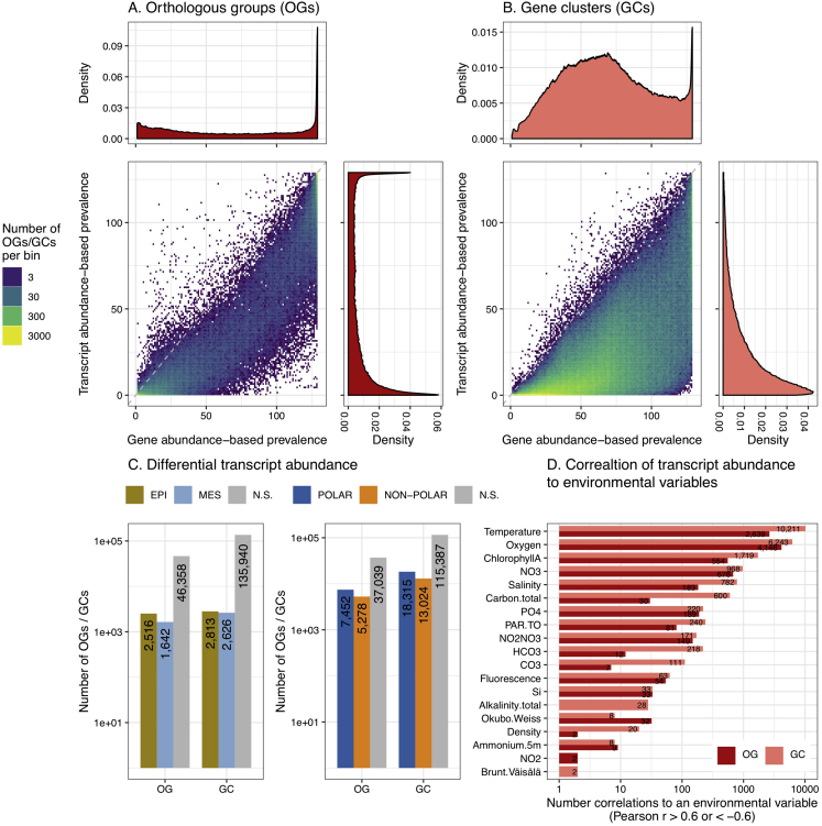
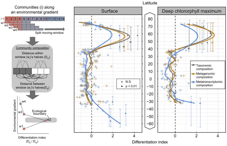
Ocean microbial communities strongly influence the biogeochemistry, food webs, and climate of our planet. Despite recent advances in understanding their taxonomic and genomic compositions, little is known about how their transcriptomes vary globally. Here, we present a dataset of 187 metatranscriptomes and 370 metagenomes from 126 globally distributed sampling stations and establish a resource of 47 million genes to study community-level transcriptomes across depth layers from pole-to-pole. We examine gene expression changes and community turnover as the underlying mechanisms shaping community transcriptomes along these axes of environmental variation and show how their individual contributions differ for multiple biogeochemically relevant processes. Furthermore, we find the relative contribution of gene expression changes to be significantly lower in polar than in non-polar waters and hypothesize that in polar regions, alterations in community activity in response to ocean warming will be driven more strongly by changes in organismal composition than by gene regulatory mechanisms. VIDEO ABSTRACT.

Keywords: Tara Oceans; biogeochemistry; community turnover; eco-systems biology; gene expression change; global ocean microbiome; metagenome; metatranscriptome; microbial ecology; ocean warming.

Graphical abstract

Figure S1

Transcript Abundance Profile as a Function of Community Composition and Gene Expression, Related to STAR Methods Cartoon exemplifying how an initial community with a given expression profile may result insimilar transcript abundance profiles through two different mechanisms: (i) changes in the community composition (upper arrow), represented by three different species (green, red, and blue), or (ii) changes in gene expression (lower arrow), represented by two different genes (purple and orange, with low and high expression levels, respectively).

Figure 1

Geographic Coverage of the Meta-omics Dataset Analyzed in This Study Geographic distribution of the sampling stations of the Tara Oceans (2009–2013) expeditions (Pesant et al., 2015). Several size-fractionated samples were collected from different depth layers at each station for a total of 557 samples (370 metagenomes and 187 metatranscriptomes). Stations numbered 155 and above represent the Tara Oceans Polar Circle campaign undertaken between June and October 2013. Colors indicate the type of samples collected for the prokaryote-enriched fractions at each station: metagenome only (orange, 18 stations); metatranscriptome only (blue, 40 stations); metagenome and metatranscriptome for at least one of the depth layers (green, 68 stations).

Figure 2

Gene Detection Rates and Annotation of the OM-RGC.v2 (A) Percentage of reads from 180 prokaryote-enriched metagenomes (orange) and 187 prokaryote-enriched metatranscriptomes (blue) aligned with a 95% identity cutoff to: the MarRef database v3, updated 2019/01/19 (Klemetsen et al., 2018), a collection of metagenome-assembled genomes (MAGs) reconstructed from Tara Oceans samples (Delmont et al., 2018), and the OM-RGC.v2 (this study). To fairly compare the alignments to the MarRef database or MAGs and the catalog, we corrected for the gene coding density in prokaryotic genomes (STAR Methods). Boxplots show the median values as horizontal lines, interquartile ranges as boxes with whiskers that extend up to 1.5 times the interquartile range, and outliers as individual data points. (B) The accumulation of OM-RGC.v2 genes detected in 180 prokaryote-enriched samples. The dashed line separates the prokaryote-enriched non-Arctic metagenomes (n = 139) (Sunagawa et al., 2015) from the Arctic metagenomes (n = 41). The increase in slope reflects an increase in the rate of detection of new genes in the Arctic Ocean. The non-prokaryote-enriched metagenomes (n = 190) and the metatranscriptomes (n = 187) are excluded from this analysis. (C) The taxonomic annotation of genes at the domain level (and viruses; LUCA, last universal common ancestor) and the breakdown of gene functional annotations into ∼9 k KEGG and ∼76 k eggNOG orthologous groups (KOs and OGs, respectively). The remaining fraction of unannotated genes was used to generate de novo gene clusters (GCs) for further functional characterization of the catalog.

Figure S2

Prevalence and Statistical Associations to the Environment of OGs and GCs, Related to STAR Methods Gene abundance-based prevalence versus transcript abundance-based prevalence (i.e., number of samples in which detected) for (A) eggNOG-based orthologous groups (OGs) and (B) de novo gene clusters (GCs) based on the 122 paired metagenomes and metatranscriptomes. Prevalence distributions are shown in the side and upper panels. The numbers of OGs and GCs with significant associations of transcript abundances to depth layers (C) and polar/non-polar regions and (D) to environmental variables are shown. Associations were detected as statistically significant differences in transcript abundance by Wilcoxon tests for depth layers and polar/non-polar regions (p < 0.05, after Holm correction for multiple comparisons) and as significant Pearson correlations for environmental variables (|r| > 0.6 and p < 0.05, after Holm correction for multiple comparisons). In both cases only the OGs and GCs with a transcript abundance-based prevalence higher than 10% were considered in order to avoid spurious associations.

Figure S3

Rationale for the Use of Co-expression Data to Associate Groups with Unknown Functions to Known Functional Groups, Related to STAR Methods Evaluation of model performance for the link between OGs based on co-variation analysis. (A) Receiver operating characteristic (ROC) curves for all models. Variation in (B) false positive rate and (C) sensitivity with increasing Pearson correlation values used as a cut-off for classification (r_min). The r_min is a value to be optimized corresponding to the minimum Pearson r that provides sufficient predictive power (false positive rate < 5%). A total of nine models are represented, which used co-abundance, co-transcription, and co-expression for the prediction of shared KEGG reactions, modules, and pathways, respectively, between pairs of OGs (see details in STAR Methods).

Figure 3

Latitudinal Partitioning of Global Ocean Microbiome Compositions The schematic on the left illustrates the underlying concept of the split moving-window analysis of ecological differentiation (Ludwig and Cornelius, 1987). It consists of a comparison of the pairwise distances between communities on opposite sides of a putative boundary with the pairwise distances between communities on the same side. A high differentiation value captures an increase in the distance between the two sides of the boundary compared with the distances within each side. The analysis was conducted with a window width of 10 samples and shows an ecological boundary centered around 60°N based on the taxonomic composition (gray, relative abundance of OTUs), metagenomic composition (orange, per-cell abundance of genes), and metatranscriptomic composition (blue, relative per-cell abundance of transcripts) of prokaryote-enriched samples from surface (SRF) and deep chlorophyll maximum (DCM) waters (both belonging to the epipelagic layer). A similar pattern is evident for the southern hemisphere; however, the limited number of samples precluded detection of an ecological boundary. Significance was determined using 99% confidence intervals computed with 10,000 random permutations of the latitude values. Vertical lines represent the window of the latitudinal range of significant values. The insufficient number of samples and latitudinal coverage prevented us to perform this analysis for the mesopelagic layer. See also Figure S4.

Figure S4

Differential Abundance of the Dominant OTUs along the Latitudinal Gradient, Related to Figure 3 Latitudinal niche value (i.e., the abundance-weighted mean absolute latitude) for the 60 most abundant OTUs in the epipelagic subset of samples. Latitudinal niche values significantly higher and lower than the value expected from a random distribution of abundances (represented by the horizontal bold lines; see STAR Methods) are color coded. The dot size is proportional to the mean relative abundance of each OTU.

Figure S5

Correlations between the Taxonomic, Metagenomic, and Metatranscriptomic Composition, Related to Figure 4 All pairwise correlations between the Euclidean distance of the (log₂-transformed) taxonomic, metagenomic, and metatranscriptomic profiles were computed for 122 samples for which all three profiles were available. The correlation strength and significance were assessed using Mantel tests with 10,000 permutations.

Figure 4

Patterns and Drivers of Global Ocean Microbiome Compositions across Depth Layers and between Polar and Non-polar Regions (A) Taxonomic, metagenomic, and metatranscriptomic composition of epipelagic samples (based on _mitags, and the normalized abundances of eggNOG-derived OGs from metagenomic and metatranscriptomic data, respectively) were related to each of 27 environmental factors using partial (geographic distance-corrected) Mantel tests with 10,000 permutations and Bonferroni correction. Pairwise comparisons of environmental factors are shown below, with a color gradient denoting Spearman’s correlation coefficients. Temperature is the best explanatory variable for all of the profiles in the epipelagic ocean (taxonomic profile: Pearson’s r = 0.75; metagenomic profile: Pearson’s r = 0.69; metatranscriptomic profile: Pearson’s r = 0.64; all p < 0.05), followed by oxygen concentration, which is highly correlated to temperature (Pearson’s r = −0.72). A more detailed description of the variables is available in https://doi.org/10.5281/zenodo.3473199. (B) Compositional richness of polar and non-polar microbiomes across three depth layers. Taxonomic and functional metagenomic richness (numbers of OTUs and OGs, respectively) increases with depth, although the richness is consistently lower in polar samples than in non-polar samples (two-way ANOVA: p < 0.05 for depth layers and polar/non-polar, for both taxonomic and metagenomic functional richness). By contrast, there was no significant difference in functional metatranscriptomic richness (number of OGs), either across depths or between polar and non-polar samples (two-way ANOVA: p > 0.05 for depth layers and polar/non-polar). Violin plots represent the (mirrored) density distribution of the data with the median shown as a horizontal line. (C) Correlations among species richness (number of OTUs), functional metagenomic (metaG) richness and metatranscriptomic (metaT) richness (number of OGs). Data were rarefied before richness computation (STAR Methods). Pearson’s correlation was used for all comparisons (OTU-metaG; r = 0.78, p < 0.001; OTU-metaT: r = 0.16, p = 0.06; metaG-metaT: r = 0.39, p < 0.05). The solid line corresponds to the best linear fit. N.S., not significant (p > 0.05). See also Figures S5 and S6.

Figure S6

Latitudinal Distribution of Seawater Temperature in the Epipelagic, Related to Figure 4 Seawater temperature (°C) measurements (n = 528) at the surface (SRF) and the deep chlorophyll maximum (DCM) along the Tara Oceans course in relation to (A) raw latitude values and (B) bins of the absolute latitude. Data are available at https://doi.org/10.1594/PANGAEA.875576.

Figure S7

Derivation of the Decomposition of a Metatranscriptome, Related to STAR Methods Mathematical basis for (A and B) the within-sample decomposition of metatranscriptomes (transcript copies / cell) into abundance (gene copies / cell) and expression (transcript copies / gene copy) components, and for (C) the between-sample decomposition of the Euclidean distance between metatranscriptomes (transcript abundance differences) into the abundance component (gene abundance differences), the expression component (expression differences), and an interaction term (abundance - expression covariation). See details in STAR Methods.

Figure 5

Differences in Gene Abundance and Expression Determine Differential Transcript Abundances of Metabolic Marker Genes across Depth Layers and between Polar and Non-polar Regions (A and B) Differences in the abundance of genes and transcripts, and the gene expression level of metabolic marker genes (KOs) were determined (A) between epipelagic and mesopelagic layers and (B) between polar and non-polar regions. The data points show the differences in the mean transcript abundances, mean gene abundances, and mean gene expression (i.e., transcript abundance normalized by gene abundance) of KOs. Differences were computed using log₂-transformed values (STAR Methods) and tested for significance by Mann-Whitney tests. Differences were considered significant if p values after Holm correction were smaller than 0.05. Only epipelagic samples were used for the data shown in (B). See also Figures S8, S9, S10, and S11.

Figure S8

Gene and Transcript Abundance of RuBisCO Subunits and PSI and PSII Marker Genes, Related to Figure 5 Distribution of whole-community (log₂-transformed) (A) gene and (B) transcript abundances of the RuBisCO subunits (rbcS and rbcL) and the marker genes for photosystem I (psaA) and II (psbA) in the epipelagic and mesopelagic depth layers. Pairwise correlations based on the (C) gene and (D) transcript abundances of the four genes are shown below. All comparisons, except the ones denoted with N.S. in (A) and (B) were significant (p < 0.05 using Wilcoxon test and Holm correction for multiple comparisons). All Pearson correlations in (B) and (C) were significant (p < 0.05).

Figure S9

Transcript Abundance of Denitrification Marker Genes along the Oxygen Gradient, Related to Figure 5 The log_2-transformed transcript abundances of nirS, norZ, nosB, and napA in relation to the oxygen concentration at the sampling location, showing a high transcript abundance in samples taken from anoxic waters (< 100 μM) and interestingly, from oxygenated waters at stations 206, 208, and 210. The depth layer (EPI or MES) and polar/non-polar nature of the sample are coded as the symbol type and color, respectively. The dot size is proportional to the concentration of NO₂ and NO₃ (μM) when available.

Figure S10

Expression and Transcript Abundance of the nifH, nifD, and nifK Genes in Relation to Nitrate and Nitrite Concentration, Related to Figure 5 Gene expression and transcript abundance of the nifH, nifD, and nifK genes in relation to the total nitrate plus nitrite concentration (μM), showing a fast decay of gene expression and transcript abundance with increased in nitrate/nitrite concentrations from 0 to 0.2 μM at absolute latitudes between 20° and 35°. Solid lines correspond to the result of local regression.

Figure 6

Relative Gene and Transcript Abundance of 24 Nitrogenase Genes (nifH) Representing nifH-Encoding “Species” (A–D) Relative gene (orange) and transcript (light blue) abundance distributions of the 24 nifH genes from the OM-RGC.v2 that were detected in 122 matched metagenomes and metatranscriptomes (A) are shown and broken down by latitude (B) and by depth (C) of the sample origin. Genes (IDs in the bottom panel) were annotated using a nifH-specific database (see STAR Methods). Boxplots in (A–C) show the median values as horizontal lines, interquartile ranges as boxes with whiskers extending up to 1.5 times the interquartile range, and all values overlaid as individual data points. Colors denote phylum-level taxonomic annotations, naming corresponds to finer grain taxonomy or database-specific identifiers (D), and stars indicate genes that were previously identified in MAGs of heterotrophic bacterial diazotrophs (HBDs) (Delmont et al., 2018). The genome containing a nifH gene for which transcripts were detected in the mesopelagic layer in the Arctic (OM-RGC.v2.019519152, bold) was reconstructed (see STAR Methods and http://doi.org/10.5281/zenodo.3352180). Horizontal dashed lines denote the latitude and depth that were used to define polar and non-polar (B) and epipelagic and mesopelagic waters (C), respectively.

Figure S11

Correlation between Assimilatory Sulfate Reduction Marker Genes and the dmdA Gene, Related to Figure 5 Transcript abundance and expression of the genes involved in the assimilatory sulfate reduction pathway in relation to the transcript abundance of the dmdA gene involved in the dimethylsulfoniopropionate (DMSP) demethylation pathway. Pearson correlation was used to test for significance of the correlation. Pearson r values and significance are shown on the plot. Log₂-transformed data were used in all cases. The correlation with the transcript abundance was significant for all genes and was especially high (−0.73) for cysD and cysN, the genes encoding the initial step of the pathway (i.e., the reduction of sulfate).

Figure S12

Temperature Dominates over Other Environmental Variables in Structuring the Relative Contribution of Community Turnover and Gene Expression Changes to Metatranscriptomic Differences between Epipelagic Communities, Related to Figure 7 Panel (A) mirrors the data in Figure 7A, so that it represents the groups of 15 samples (bins) along the temperature gradient on the x axis. The y axis, however, captures the distribution of the temperature differences within each bin. Notably, the distributions of these differences are highly similar in polar and non-polar waters. This indicates that the higher relative contribution of turnover in polar waters and gene expression changes in non-polar waters occurs for a similar range of temperature differences. (B) The distribution of the interaction component (see Equation 1 in STAR Methods) for all the polar-to-polar and non-polar-to-non-polar comparisons across the bins are not significantly different from each other (Wilcoxon test), which indicates that the absolute values of turnover and gene expression changes are comparable between polar and non-polar communities (Figure 7B). Panel (C) is based on Figure 7A and serves as an explanatory schematic for panel (D). To evaluate the influence of an environmental parameter on the relative contribution of community turnover and gene expression changes, a similar analysis to the one in Figure 7A was performed. A score was attributed to each parameter as the sum of the deviation of each bin from 1 (where the effect of both mechanisms is identical). The deviation of each individual bin is visualized as a gray line. The results are summarized in panel (D) for the environmental parameters that were tested. The vertical lines indicate the distribution of this score for 100 random binnings (solid line denotes the median value and dashed lines represent the 95% interval of the distribution). As a result, we identify that daylength, temperature and chlorophyll concentrations have significant effects on the relative contributions. We further investigated these parameters, by assessing the distribution of environmental variation for polar and non-polar regions across the bins [panels (E), (G), and (I)], and the relationship between the relative contributions (of community turnover and gene expression changes) and the variation in the environmental parameter across the whole (unbinned) dataset [panels (F), (H), and (J)]. The left-side [(E), (G), and (I)] aims at answering whether the difference in regimes that are observed between polar and non-polar regions may simply be due to a different range of environmental variation. The distributions display little differences in the case of temperature, while they are strongly contrasted for daylength and chlorophyll concentrations. Furthermore, (F), (H), and (J) provide a direct estimation of the relationship of the relative contributions of community turnover and gene expression changes with the environmental distance. Based on linear models, temperature differences capture most of the variance, both in polar and non-polar regions. In contrast, daylength and chlorophyll concentrations show a weaker or no trend, especially in polar regions (despite a wide range of variation). Overall, this confirms that among the parameters tested, temperature is the best explanatory variable for the difference in the relative contribution of community turnover and gene expression changes observed between polar and non-polar epipelagic communities.

Figure 7

Relative Contributions of Community Turnover and Gene Expression Changes to Variations in Metatranscriptome Composition Determination of the relative contributions of community turnover and gene expression changes to variations in the metatranscriptome composition requires the decomposition of metatranscriptomic distances between communities (Figure S7; STAR Methods). Specifically, the relative contribution is determined as the ratio of the gene abundance-based distance (community turnover) and the gene expression-based distance (gene expression changes) between two metatranscriptomes. (A) The relationship of the ratio with temperature was analyzed by dividing the epipelagic samples into groups (bins) of 15 samples each using a sliding window along the temperature gradient. For each bin, we report the median ratio (among all the pairwise comparisons within each bin) as a function of the median temperature of the samples present in the bin. The significance is determined by a Wilcoxon test comparing the within-bin distribution of the ratios to 1 (in which case the relative contributions of community turnover and gene expression changes are the same). The Holm correction was used to adjust for multiple testing. The ratio was considered to be significantly different from 1 if p < 0.05. (B) The inner panel represents the difference for community turnover and gene expression changes between polar and non-polar regions. The distributions capture the distances of each component for all pairwise comparisons of polar and non-polar epipelagic samples. Violin plots represent the (mirrored) density distribution of the data with the median shown as horizontal line. Significance was tested by the Wilcoxon test; ^∗∗∗p < 0.001. See also Figure S12.

References

1. Alberti A., Belser C., Engelen S., Bertrand L., Orvain C., Brinas L., Cruaud C., Giraut L., Da Silva C., Firmo C. Comparison of library preparation methods reveals their impact on interpretation of metatranscriptomic data. BMC Genomics. 2014;15:912. - PMC - PubMed
1. Alberti A., Poulain J., Engelen S., Labadie K., Romac S., Ferrera I., Albini G., Aury J.-M., Belser C., Bertrand A., Genoscope Technical Team. Tara Oceans Consortium Coordinators Viral to metazoan marine plankton nucleotide sequences from the Tara Oceans expedition. Sci. Data. 2017;4:170093. - PMC - PubMed
1. Alexander M.A., Scott J.D., Friedland K.D., Mills K.E., Nye J.A., Pershing A.J., Thomas A.C. Projected sea surface temperatures over the 21st century: Changes in the mean, variability and extremes for large marine ecosystem regions of Northern Oceans. Elem. Sci. Anth. 2018;6:9.
1. Almeida A., Mitchell A.L., Boland M., Forster S.C., Gloor G.B., Tarkowska A., Lawley T.D., Finn R.D. A new genomic blueprint of the human gut microbiota. Nature. 2019;568:499–504. - PMC - PubMed
1. Anderson R., Mawji E., Cutter G., Measures C., Jeandel C. GEOTRACES: Changing the Way We Explore Ocean Chemistry. Oceanography. 2014;27:50–61.
LinkOut - more resources