Global Trends in Marine Plankton Diversity across Kingdoms of Life

Abstract

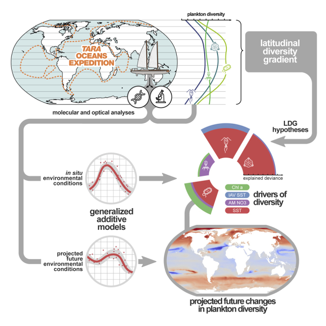
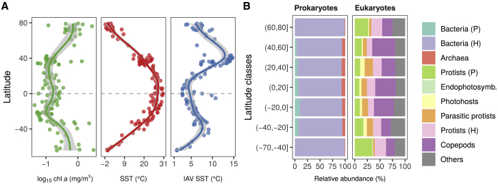
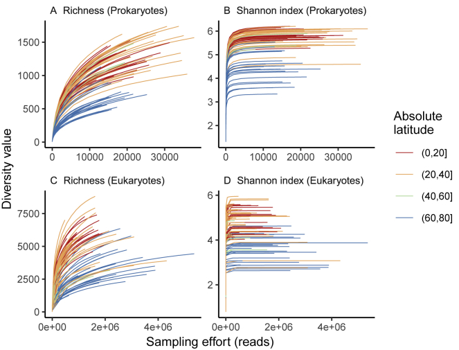
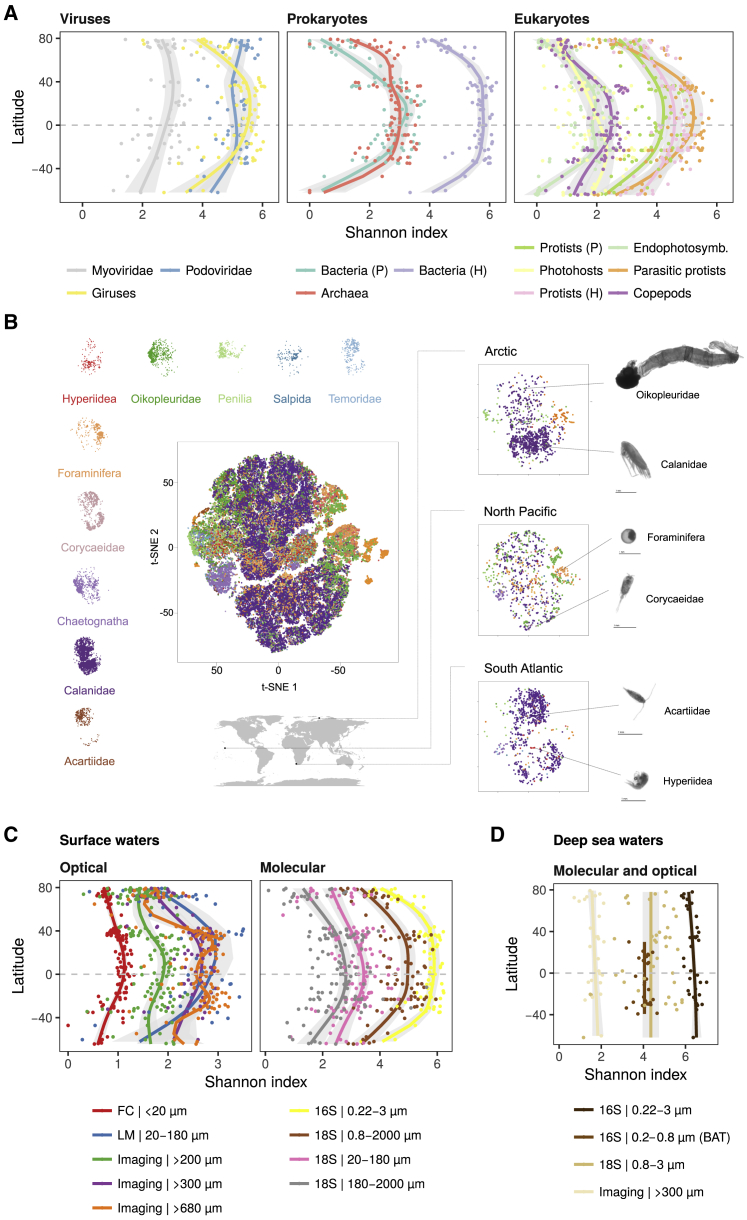
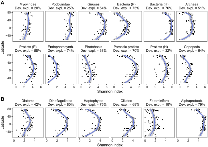
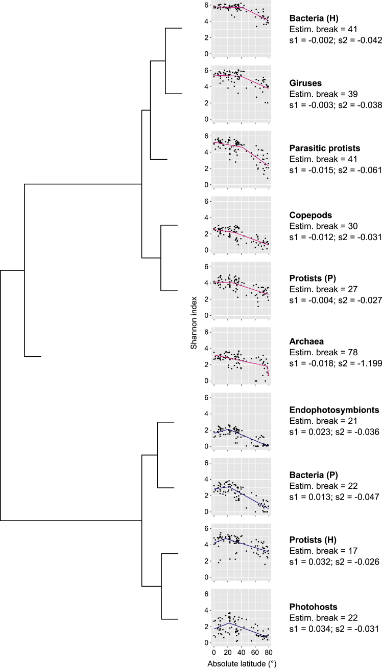
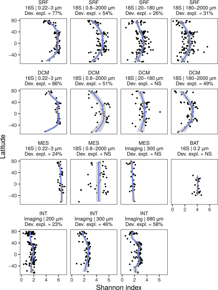
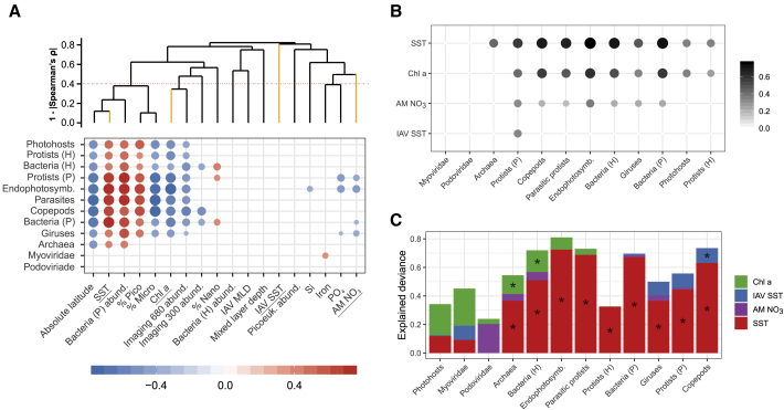
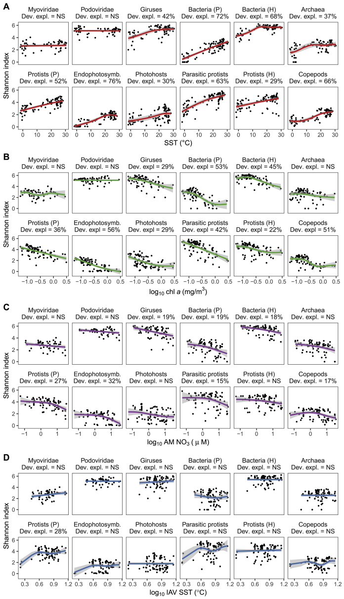
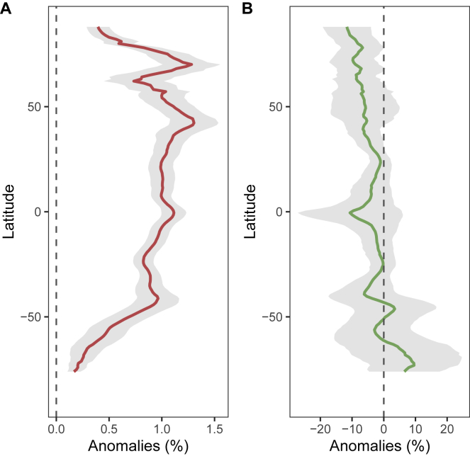
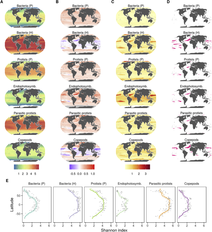
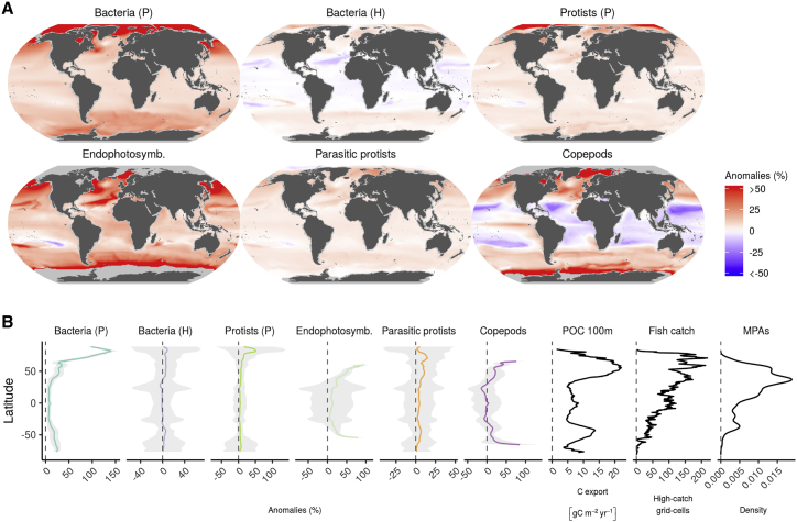
The ocean is home to myriad small planktonic organisms that underpin the functioning of marine ecosystems. However, their spatial patterns of diversity and the underlying drivers remain poorly known, precluding projections of their responses to global changes. Here we investigate the latitudinal gradients and global predictors of plankton diversity across archaea, bacteria, eukaryotes, and major virus clades using both molecular and imaging data from Tara Oceans. We show a decline of diversity for most planktonic groups toward the poles, mainly driven by decreasing ocean temperatures. Projections into the future suggest that severe warming of the surface ocean by the end of the 21^st century could lead to tropicalization of the diversity of most planktonic groups in temperate and polar regions. These changes may have multiple consequences for marine ecosystem functioning and services and are expected to be particularly significant in key areas for carbon sequestration, fisheries, and marine conservation. VIDEO ABSTRACT.

Keywords: Tara Oceans; climate warming; high-throughput imaging; high-throughput sequencing; latitudinal diversity gradient; macroecology; plankton functional groups; temperature; trans-kingdom diversity.

Graphical abstract

Figure 1

Latitudinal Trends of Oceanic Conditions and Marine Plankton Composition in Surface Waters (A) In situ chl a concentrations and sea surface temperatures (SST) across latitude (Tara Oceans expedition), plus IAV of SST (STAR Methods). Solid lines represent the GAM smooth trends and gray ribbons the corresponding 95% confidence intervals of parameter latitudinal trends predicted by the GAMs. (B) Average relative abundances of MPGs as inferred from molecular datasets across latitude. Prokaryotes: 16S rRNA gene, 0.22–3 μm; eukaryotes: 18S rRNA gene, 0.8–2000 μm (STAR Methods). Dark gray represents other eukaryotic groups. P, photosynthetic/mixotrophic; H, non-photosynthetic/heterotrophic. The three viral groups are not represented here because of the absence of comparable abundance data. See also Figures S1 and S2 and Tables S1A and S1B.

Figure S1

Tara Oceans Stations and Shannon Diversity Patterns, Related to Figures 1 and 2 (A) MPGs at the sea surface (< 5 m depth), (B) whole planktonic community using different sampling protocols at the sea surface (except for “Imaging,” integrative depth from 500 m depth to the surface) and (C) whole planktonic community of the mesopelagic realm (200-1000 m depth). Number of stations are specified in the inset titles. Color represents the Shannon index. For more details on the different size fractions and sampling protocols, please refer to the caption in Figure 1 and STAR Methods.

Figure S2

Average Abundances of a Broader List of Plankton Groups across Latitude, Related to Figures 1 and 2 For 18S rDNA metabarcodes (relative abundances), imaging from net catches and flow cytometry (absolute abundances). Numbers refer to the filter mesh size (μm). H: non-photosynthetic/heterotrophic, P: photosynthetic/mixotrophic. See Figures 1 and S1 for further sampling details. The three viral groups are not represented here due to absence of comparable abundance data. Note that the differences between protocols relate, among other things, to resolution (e.g., potential photohosts from the nets are classified as Protists (H)), marker gene copy number (e.g., high in photohosts), lack of detection (many small copepods are lost when sampling with nets), or water column sampling differences (surface [SRF] or deep chlorophyll maximum [DCM] versus integrative [INT] for molecular/cytometry versus net catches, respectively).

Figure S3

Rarefaction Curves for the Plankton Community, Related to Figure 2 and STAR Methods Based on richness (A, C) and Shannon (B, D), for prokaryotes (16S rRNA gene miTags, A, B), and eukaryotes (18S rRNA gene V9 metabarcoding, C, D). Each line corresponds to a surface water sample. Colors correspond to different latitudinal bands (absolute values).

Figure 2

Latitudinal Patterns of Marine Plankton Diversity (A) LDGs at the sea surface for all MPGs (STAR Methods). (B) Morphological diversity as analyzed from more than 77,000 organisms collected with the bongo net (imaging | 300 μm). Morphological measurements were normalized and subjected to a t-distributed stochastic neighbor embedding (t-SNE) ordination analysis using all samples (STAR Methods). In the central 2D t-SNE ordination, each dot corresponds to an organism and its color to its taxonomic assignation (>100 taxa). For ease of interpretation, the points corresponding to a subset of abundant groups are displayed separately. The three t-SNE ordinations displayed on the right show dots from three stations distantly located and from different latitudes, as shown in the map. Six images are also presented as examples of the underlying data (STAR Methods); 1-mm scale bars are shown below each picture. (C and D) Patterns of the whole plankton community using different sampling protocols at (C) the sea surface (16S/18S/FC/LM) or a larger integrative depth of 500 m (imaging) and (D) in mesopelagic (average depth, 540 m) or bathypelagic layers (BAT; average depth, 4000 m, Malaspina expedition). In all cases, solid lines correspond to GAM smooth trends and gray ribbons to the 95% confidence intervals of the Shannon latitudinal trend predicted by the GAMs (see also Figures S4 and S7 for individual curves and explained deviance). These trends are drawn for illustrative purposes and were not used in downstream analyses. 16S and 18S refer to the different rRNA subunit genes used as marker genes for metagenomics and metabarcoding, respectively. Imaging refers to the identification method for large eukaryotes captured with nets. FC refers to flow cytometry for the picoplankton and LM to the light microscopy-based survey of microphytoplankton (STAR Methods). Numbers refer to the filter mesh size.

Figure S4

Sea Surface LDG, Related to Figure 2A (A) For viral, prokaryotic and eukaryotic MPGs, and (B) for well-known protist phyla and the dominant class of bacteria, Alphaproteobacteria, for which ∼50% corresponds to the SAR11 clade. Solid lines represent the GAM smooth trends and gray ribbons the corresponding 95% confidence intervals of the Shannon latitudinal trend predicted by the GAMs. The percentages provided below inset titles correspond to the deviance explained by GAMs when significant. Viruses and bacterial diversities are inferred from samples filtered at 0.22-3 μm and analyzed through marker genes derived from metagenomics. Eukaryote diversity shown here is inferred from 18S rDNA metabarcoding of samples filtered at 0.8-2000 μm. H: non-photosynthetic/heterotrophic, P: photosynthetic/mixotrophic.

Figure S5

Classification of MPG Sea Surface LDG Analyzed by Segmented Regression, Related to Figure 2A The estimated break is the absolute latitude between the two segments of slope s₁ and s₂, respectively. We used pink lines for s₁ ≤ 0 (plateau or peak around the equator) and blue lines for s₁ > 0 (extra-equatorial peak). The dendrogram is the result of a hierarchical clustering based on the differences in break and slope values across MPGs (Euclidean distance on standardized values).

Figure S6

Correlation between the Shannon Values Derived from Multiple Datasets of Tara Oceans, Related to STAR Methods (A) OTUs (as defined with “swarm”; Mahé et al., 2014) obtained with the V9 (x axis) and V4 (y axis) regions of the 18S rRNA gene using surface water samples (SRF); size fraction 0.8-2000 μm; (B) OTUs either as defined with swarm (x axis) or defined at 100% sequence identity from the V9 region of the 18S rRNA gene for SRF samples, size fraction 0.8-2000 μm; (C-D) 16S rRNA gene miTags (x axis) versus OTUs defined at 97% [C] and 100% sequence similarity [D] (y axis) obtained from the V4-V5 regions of the 16S rRNA gene for SRF samples, size fraction 0.22-3 μm. (E) OTUs of photosynthetic protists obtained with the V9 region of the 18S rRNA gene (x axis) versus protists (mostly photosynthetic) as identified with environmental High Content Fluorescence Microscopy (eHCFM; data from Colin et al., 2017) in SRF-DCM samples, size fraction 5-20 μm; (F) Diatom OTUs obtained with V9 region of the 18S rRNA gene (x axis) versus diatom species counted by light microscopy (y axis) in SRF samples; size fraction 20-180 μm; (G/H) Copepod OTUs obtained with the V9 region of the 18S rRNA gene, SRF samples, size fraction 180-2000 μm (x axis) versus abundances [G] and biovolumes [H] of copepods collected by the WP2 net, > 200 μm. Inset titles show the Pearson’s correlation coefficient and its associated p value. Note the differences in axes scales. Dashed line represents 1:1 relation. Refer to STAR Methods for details on each method.

Figure S7

LDG across Size and Depth, Related to Figures 2B–2D For the whole prokaryotic (16S miTags, 0.22-3 μm, and 16S OTUs, 0.2 μm for bathypelagic (BAT)) and eukaryotic communities (18S OTUs, 0.8-2000, 20-180 and 180-2000 μm; imaging, > 300 and > 680 μm) at different depths (SRF: surface, < 5 m; DCM: deep chlorophyll maximum, 17-188 m, and MES: mesopelagic, > 200 m, BAT: bathypelagic, > 4000 m, INT: integrative, depth from 500 m depth to the surface). Non-significant GAMs are denoted with “NS.” See Figure S4 legend for more information on the plot. Note that the particular trend for the regent net, i.e., Imaging | 680 μm might be due to undersampling of small zooplankton.

Figure S8

Multiple Pairwise Spearman Correlation Analysis of the Full Matrix of Contextual Parameters for the Surface Ocean, Related to Figure 3A Rows and columns were clustered based on the absolute pairwise Spearman correlation turned into distance (1 - |⍴|). MLD: mixed layer depth. E_median ML: median light in the mixed layer. IAV: intra-annual variability. Part.backscat.coef: particle backscattering coefficient. For more information on parameters, see Figure 3 and STAR Methods.

Figure 3

Drivers of Plankton Diversity in the Surface Ocean (A) Correlation of contextual variables (abiotic and population densities, x axis) with the Shannon index of each MPG (y axis). The color gradient corresponds to the values of the Spearman ρ correlation coefficient and the dot size to their absolute value. The labels of the x axis are ordered according to a hierarchical clustering analysis of absolute Spearman ρ correlation coefficient values between each pair of contextual variables, whose corresponding dendrogram is shown in the top part of the plot. Yellow leaves correspond to the four variables analyzed in (B) and (C), also underlined below. Variables that do not cluster above the dotted line (|Spearman’s ρ| < 0.6) are considered as non-collinear. Percentages of pico, nano, and micro refer to the relative abundances of fractions of phytoplankton based on pigment analysis. Bacteria and picoeukaryote abundances were determined by FC, whereas imaging abundances refer to counts of individuals caught by nets (STAR Methods). MLD: mixed-layer depth. See also Figure S8. (B and C) Individual explained deviance (color gradient and dot size) of four variables (B; Figure S9) and additive contribution of the same four variables to the total explained deviance in GAMs, with the Shannon index as a response variable (C; STAR Methods; Tables S1D and S1E). In (A) and (B), non-significant coefficients or effects are not shown. In (C), significant effects are indicated by asterisks. MPG labels are always ordered according to a hierarchical clustering analysis after a Spearman correlation analysis based on the displayed values in each case (A–C).

Figure S9

Relationships between Diversity and 4 Contextual Variables for Viral, Prokaryotic, and Eukaryotic MPGs, Related to Figure 3B (A) SST, (B) chl a, (C) AM NO₃, and (D) IAV SST. Solid lines represent the GAM smooth trends and gray ribbons the corresponding 95% confidence intervals of the x-y relationship predicted by the GAMs. The percentages provided below inset titles correspond to the deviance explained by GAMs when significant (p value corrected for multiple comparisons). Non-significant GAMs are denoted with “NS.”

Figure S10

Relationship between Plankton Abundance and Two Contextual Variables, Related to Figure 3A (A) SST, (B) chl a. Abundance values were obtained with flow cytometry (reported in [cells/ml]) or from counts of individuals captured with nets of different mesh size and identified by imaging (reported in [individuals/m³]), respectively. Solid lines represent the GAM smooth trends and gray ribbons the corresponding 95% confidence intervals of the X-Y relationship predicted by the GAMs. The percentages provided below inset titles correspond to the deviance explained by GAMs when significant.

Figure S11

Projected Latitudinal Changes in SST and chl a, Related to Figures 4 and S12 Anomalies (%) in (A) SST and (B) chl a at the end of the 21st century (2090-2099, RCP 8.5) relative to the beginning of the century (1996-2006). Data was obtained from 13 CMIP5 models (Table S1H). Grey ribbons represent the standard error.

Figure S12

Modeled Patterns of Diversity of MPGs in the Global Ocean, Related to Figure 4 (A) Shannon index modeled at the global scale for oceanic conditions at the beginning of the 21st century (1996-2006). Predicted Shannon values ≤ 0 obtained at high latitudes, particularly for copepods and endophotosymbionts, were excluded. (B) Anomalies were calculated as the difference of their Shannon index at the end (2090-2099, RCP 8.5) and the beginning of the century (1996-2006). A positive value means that diversity will increase by the end of the century. Note that the scale is not symmetric and that white means zero change. (C) Uncertainty maps (standard deviation) for (B). (D) Areas where the effect of chl a on plankton diversity is likely to be higher than the one of SST. To determine this, either chl a or SST were held constant in the projections by the end of the century. Then, if the anomaly caused only by the change of chl a was different than zero and higher (absolute terms) than the one caused only by the change in SST, the pixel was colored. (E) Latitudinal diversity gradient at the beginning (solid line) and the end (dashed line) of the 21st century. Values represent averages over longitude for each latitudinal degree. Dots are observed values (Figure 2). 13 Earth system models from CMIP5 were used (Table S1H).

Figure 4

Projected Changes in Shannon Diversities by the End of the 21^st Century (A) Projected changes by the end of the 21^st century relative to the beginning of the century (percent) for MPGs accounting for GAM models with high explained deviance (>60%). Projections were based on SST and chl a data simulated by the CMIP5 models and the GAMs (n = 13,000 for each combination of MPG and time frame; STAR Methods; Tables S1F–S1H; see Figure S12 for SD by grid cell). Copepods, photosynthetic protists, parasitic protists, and endophotosymbiont diversity (Shannon index) was modeled based on 18S rRNA gene metabarcoding data, size fraction 0.8–2000 μm, and diversity of heterotrophic and photosynthetic bacteria on 16S rRNA gene metagenomics data (size fraction 0.22–3 μm), all from the surface layer. Predicted Shannon values of 0 or less obtained at high latitudes, particularly for copepods and endophotosymbionts, were excluded. (B) Latitudinal averages of values in (A) and their uncertainties. For visualization purposes, average anomalies for endophotosymbionts and copepods were drawn up to latitudes where values remain below 100%, and all plots show the averaged SD reduced by half. The x axis is not fixed. The last three panels refer to latitudinal averages of particulate organic carbon (POC) export at 100 m (Henson et al., 2012), the number of grid cells with a high marine fisheries catch (>200 kg km⁻² year⁻¹) (Watson, 2017), and marine protected area (MPA) latitude kernel density plots (Bruno et al., 2018; STAR Methods; Table S1I).

Figure S13

Correlation between the Shannon Values Observed in Independent Datasets and Those for the Same Locations that Are Predicted by GAM Models Built in This Work, Related to STAR Methods (A) Heterotrophic bacteria from the surface, open ocean water sites of the International Census of Marine Microbes (ICoMM; Zinger et al., 2011). (B) Eukaryotic community retrieved from Raes et al. (2018). Note that for the latter the mesh size of the filters used were not exactly the same (Tara Oceans > 0.8 μm; Raes et al., 2018 > 0.22 μm). Note also that both datasets have different sampling dates and locations in relation to Tara Oceans. In both cases we used as predictors the temperature and chl a of each site predicted by 13 CMIP5 models at the month of sampling averaged over 1996-2006. Inset titles show the Pearson’s correlation coefficient and its associated p value.

References

1. Adriaenssens E.M., Cowan D.A. Using signature genes as tools to assess environmental viral ecology and diversity. Appl. Environ. Microbiol. 2014;80:4470–4480. - PMC - PubMed
1. Alberti A., Poulain J., Engelen S., Labadie K., Romac S., Ferrera I., Albini G., Aury J.-M., Belser C., Bertrand A., Genoscope Technical Team. Tara Oceans Consortium Coordinators Viral to metazoan marine plankton nucleotide sequences from the Tara Oceans expedition. Sci. Data. 2017;4:170093. - PMC - PubMed
1. Algar A.C., Kharouba H.M., Young E.R., Kerr J.T. Predicting the future of species diversity: macroecological theory, climate change, and direct tests of alternative forecasting methods. Ecography. 2009;32:22–33.
1. Allen A.P., Gillooly J.F., Savage V.M., Brown J.H. Kinetic effects of temperature on rates of genetic divergence and speciation. Proc. Natl. Acad. Sci. USA. 2006;103:9130–9135. - PMC - PubMed
1. Aminot A., Kérouel R., Coverly S. Nutrients in Seawater Using Segmented Flow Analysis. In: Wurl O., editor. Practical Guidelines for the Analysis of Seawater. Taylor & Francis; 2009.