Learning optimal decisions with confidence

Abstract

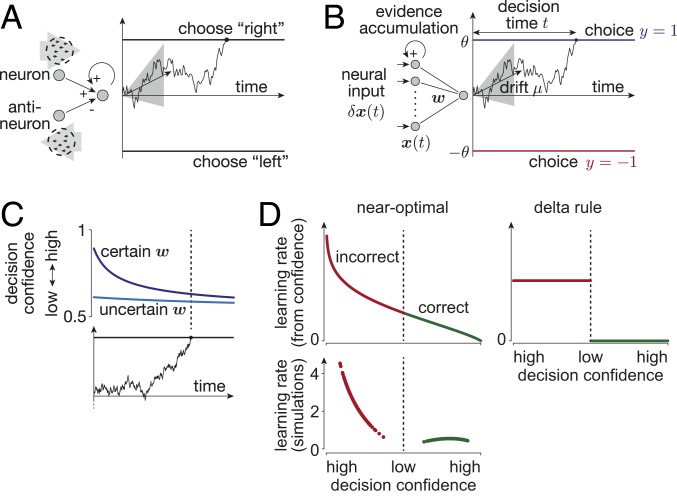
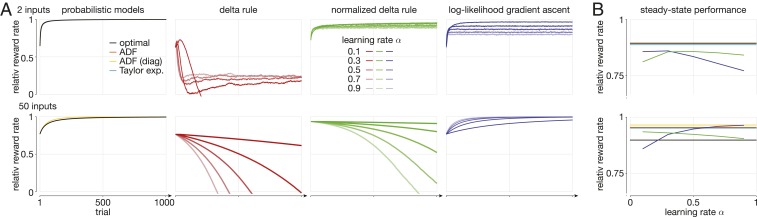
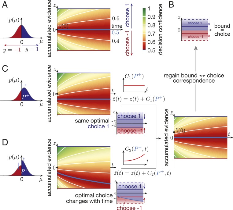
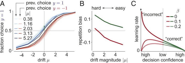
Diffusion decision models (DDMs) are immensely successful models for decision making under uncertainty and time pressure. In the context of perceptual decision making, these models typically start with two input units, organized in a neuron-antineuron pair. In contrast, in the brain, sensory inputs are encoded through the activity of large neuronal populations. Moreover, while DDMs are wired by hand, the nervous system must learn the weights of the network through trial and error. There is currently no normative theory of learning in DDMs and therefore no theory of how decision makers could learn to make optimal decisions in this context. Here, we derive such a rule for learning a near-optimal linear combination of DDM inputs based on trial-by-trial feedback. The rule is Bayesian in the sense that it learns not only the mean of the weights but also the uncertainty around this mean in the form of a covariance matrix. In this rule, the rate of learning is proportional (respectively, inversely proportional) to confidence for incorrect (respectively, correct) decisions. Furthermore, we show that, in volatile environments, the rule predicts a bias toward repeating the same choice after correct decisions, with a bias strength that is modulated by the previous choice's difficulty. Finally, we extend our learning rule to cases for which one of the choices is more likely a priori, which provides insights into how such biases modulate the mechanisms leading to optimal decisions in diffusion models.

Keywords: confidence; decision making; diffusion models; optimality.

Fig. 1.

Learning the input weights from feedback in diffusion models. In diffusion models, the input(s) provide at each point in time noisy evidence about the world’s true state, here given by the drift $\mu$. The decision maker accumulates this evidence over time (e.g., black example traces) to form a belief about $\mu$. Bayes-optimal decisions choose according to the sign of the accumulated evidence, justifying the two decision boundaries that trigger opposing choices. (A) In standard diffusion models, the momentary evidence either arises directly from noisy samples of $\mu$, or, as illustrated here, from a neuron/antineuron pair that codes for opposing directions of evidence. The illustrated example assumes a random-dot task, in which the decision maker needs to identify whether most of the dots that compose the stimulus are moving either to the left or to the right. The two neurons (or neural pools) are assumed to extract motion energy of this stimulus toward the right (Top) and left (Bottom), such that their difference forms the momentary evidence toward rightward motion. A decision is made once the accumulated momentary evidence reaches one of two decision boundaries, triggering opposing choices. (B) Our setup differs from that in A in that we assume the input information $\delta \mathit{x}\left(t\right)$ to be encoded in a larger neural population whose activity is linearly combined with weights $\mathit{w}$ to yield the one-dimensional momentary evidence, and that the decision maker aims to learn these weights from feedback about the correctness of her choices. (C) Decision confidence (i.e., the belief that the made choice was correct) in this kind of diffusion model drops as a function of time (horizontal axis) and with increased uncertainty about the input weights (different shades of blue). (D) For near-optimal learning, the learning rate (the term ${\xi }_w$ in Eq. 6) is modulated by decision confidence (Top Left). High-confidence decisions lead to little learning if correct (green, Right), and strong learning if incorrect (red, Left). Low-confidence decisions result in a moderate confidence-related learning rate term (Top and Center). The learning rate in 1,000 simulated trials (Bottom) shows that the overall learning rate preserves this trend, with an additional suppression of learning for low-confidence decisions. Other learning heuristics (e.g., the delta rule, Right) do not modulate their learning by confidence.

Fig. 2.

Input weight learning and tracking performance of different learning rules. All plots show the relative reward rate (0 = immediate, random choices; 1 = optimal) averaged over 5,000 simulations with different true, underlying weights, and for 2 (Top) and 50 (Bottom) inputs. (A) The relative reward rate for probabilistic and heuristic learning rules. The probabilistic learning rules include the optimal rule (Gibbs sampling), assumed density filtering (ADF), ADF with a diagonal covariance matrix (ADF [diag]), and a learning rule based on a second-order Taylor expansion of the log-posterior (Taylor exp.). For both 2 and 50 inputs, all rules perform roughly equally. For the heuristic rules, different color shadings indicate different learning rates. The initial performance shown is that after the first application of the learning rule, such that initial performances can differ across learning rules. (B) The steady-state performance across different heuristic rule learning rates. Steady-state performance was measured as an average across 5,000 simulations, averaging over the last 100 of 1,000 simulated trials in which the true weights slowly change across consecutive trials. An optimal relative reward rate of 1 corresponds to knowing the true weight in each trial, which, due to the changing weight, is not achievable in this setup. The color scheme is the same as in A, but the vertical axis has a different scale. The delta rule did not converge and was not included in B.

Fig. 3.

Decision confidence, prior biases, and the relation between decision boundary and choice. (A) For an unbiased prior [i.e., $P^{+}\equiv p\left(\mu \ge 0\right)=1/2$], the decision confidence (color gradient) is symmetric around $z=0$ for each fixed time $t$. The associated posterior belief $p\left(\mu \ge 0|z\left(t\right),t\right)$ (numbers above/below “time” axis label; constant along white lines; $\mathrm{½}$ along light blue line) promote choosing $y=1$ and $y=-1$ above (blue area in B) and below (red area in B) $z=0$. (B) As a result, different choices are Bayes-optimal at the blue/red decision boundaries, as long as they are separated by $z=0$, irrespective of the boundary separation (solid vs. dashed blue red lines). (C) If the prior is biased by an overall shift, the decision confidence is countershifted by the same constant across all $t$. In this case, both decision boundaries might promote the same choice, which can be counteracted by a time-invariant shift of $z$ by $C_1\left(P^{+}\right)$. (D) If the prior is biased by boosting one side while suppressing the other, the decision confidence shift becomes time dependent, such that the optimal choice at a time-invariant boundary might change over time. Counteracting this effect requires a time-dependent shift of $z$ by $C_2\left(P^{+},t\right)$. In both C and B, we have chosen $P^{+}=0.6$, for illustration.

Fig. 4.

Sequential choice dependencies due to continuous learning, and effects of noisy feedback. Bayes-optimal learning in a slowly changing environment predicts sequential choice dependencies with the following pattern. (A) After hard, correct choices (low prev. $\left|\mu \right|$; light colors), the psychometric curve is shifted toward repeating the same choice (blue/red = choice $y=1/-1$). This shift decreases after easier, correct choices (high prev. $\left|\mu \right|$; dark colors). (B) We summarize these tuning curve shifts in the repetition bias, which is the probability of repeating the same choice to a $\mu =0$ stimulus (example green arrow for $\mu =-0.38$ in A). After correct/incorrect choices (green/red curve), this leads to a win–stay/lose–switch strategy. Only the win–stay strategy is shown in A. (C) If choice feedback is noisy (inverted with probability $\beta$), the learning rate becomes overall lower. In particular for high-confidence choices with “incorrect” feedback, the learning rate becomes zero, as the learners trust their choice more than the feedback.

References

1. Doya K., Ishii S., Pouget A., Rao R. P. N., Bayesian Brain: Probabilistic Approaches to Neural Coding (MIT Press, 2006).
1. Ratcliff R., A theory of memory retrieval. Psychol. Rev. 85, 59–108 (1978).
1. Ratcliff R., McKoon G., The diffusion decision model: Theory and data for two-choice decision tasks. Neural Comput. 20, 873–922 (2008). - PMC - PubMed
1. Bogacz R., Brown E., Moehlis J., Holmes P., Cohen J. D., The physics of optimal decision making: A formal analysis of models of performance in two-alternative forced-choice tasks. Psychol. Rev. 113, 700–765 (2006). - PubMed
1. Ratcliff R., Smith P. L., A comparison of sequential sampling models for two-choice reaction time. Psychol. Rev. 111, 333–367 (2004). - PMC - PubMed
Publication types
LinkOut - more resources