Learning from methylomes: epigenomic correlates of Populus balsamifera traits based on deep learning models of natural DNA methylation

Abstract

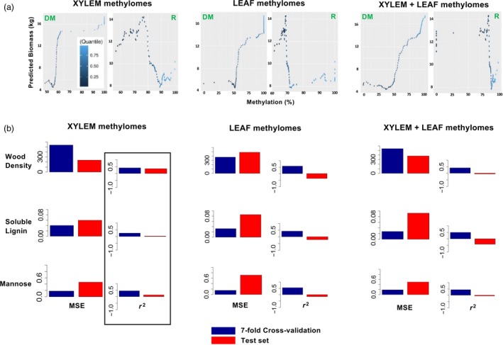
Epigenomes have remarkable potential for the estimation of plant traits. This study tested the hypothesis that natural variation in DNA methylation can be used to estimate industrially important traits in a genetically diverse population of Populus balsamifera L. (balsam poplar) trees grown at two common garden sites. Statistical learning experiments enabled by deep learning models revealed that plant traits in novel genotypes can be modelled transparently using small numbers of methylated DNA predictors. Using this approach, tissue type, a nonheritable attribute, from which DNA methylomes were derived was assigned, and provenance, a purely heritable trait and an element of population structure, was determined. Significant proportions of phenotypic variance in quantitative wood traits, including total biomass (57.5%), wood density (40.9%), soluble lignin (25.3%) and cell wall carbohydrate (mannose: 44.8%) contents, were also explained from natural variation in DNA methylation. Modelling plant traits using DNA methylation can capture tissue-specific epigenetic mechanisms underlying plant phenotypes in natural environments. DNA methylation-based models offer new insight into natural epigenetic influence on plants and can be used as a strategy to validate the identity, provenance or quality of agroforestry products.

Keywords: authentication; deep learning; epigenomics; poplar.

Figure 1

Study design and phenotyping of natural Populus balsamifera populations grown in two common gardens. (a) Schematic illustration of the study design. Twenty‐five P. balsamifera genotypes were replicated between two field sites, Indian Head and Prince Albert, Saskatchewan, Canada. Three‐letter code indicates the provenance of the trees from which germplasm was sampled (see Methods). The number assigned to each tree represents a distinct genotype within a provenance. Genotypes in purple boxes comprise the test set on which phenotypic predictions were evaluated. (b) Box plots of tree biomass, wood density, soluble lignin content and mannose content after 6 years of growth. Trees are grouped by provenance, and letters indicate significant differences among groups according to Tukey’s HSD test.

Figure 2

Exploratory analyses of CpG methylation in the training set. Genome‐wide patterns of CpG methylation in 72 methylomes comprising the training set. (a) Pearson’s correlation coefficient calculated on each pairwise combination of methylomes, using the set of 12358704 CpG covered by sequencing. (b) PCA conducted using this set of CpG. Distribution of methylomes is presented along PC1 and PC2 axes (left) and along PC3 and PC4 axes (right). Colour scale indicates contribution of methylomes to principal components. (c) Hierarchical clustering conducted on 200,000 randomly selected CpG using the Ward clustering method on Euclidean distances. Rectangles surround clusters supported at 0.95 level of significance. p‐Values denoted in green are estimated as bootstrap probabilities (bp) calculated using 1,000 bootstrap iterations. p‐Values denoted in red are approximately unbiased (au). (d) t‐SNE representation in 3 dimensions, calculated with the same 200,000 CpG used in (c).

Figure 3

Variable selection and deep learning models classifying tissue type. (a) Schematic illustration of the differential methylation strategy used on 72 methylomes comprising the training set. (b) Differential methylation calculated using Welch’s t‐test on the training set at α = 0.01 level of significance and FDR at increasing levels of stringency. (c) Summary statistics of model fit and performance after sevenfold cross‐validation of the training set and on test set predictions. Cytosines used in modelling were either 8,400 CpG selected by differential methylation, 14 CpG selected by further backward elimination or 14 CpG randomly selected. MSE denotes mean squared error, and error denotes the misclassification rate. (d) Variable selection by backward elimination. Each of the 8,400 CpG used in the initial tissue prediction model is plotted according to its variable importance (open circles). Arrows indicate the number of CpG selected for modelling according to variable importance calculated in successively smaller models.

Figure 4

Interpretation of a model classifying tissue based on methylation of 14 CpG. (a) Neural interpretation diagram. I—input neuron, O—output neuron, H—hidden neuron, B—bias neuron. Red—stimulatory connection, blue—inhibitory connection. Line width is proportional to the magnitude of the connection. Input neurons are shaded from bright to dark green according to diminishing variable importance. (b) Methylation‐response plots illustrating the relationship between cytosine methylation level and the probability associated with each tissue. For each of the 14 CpG, points are plotted separately by tissue class (left), and for both tissue classes together (right).

Figure 5

Variable selection and deep learning models classifying poplar provenances. (a) Schematic of differential methylation tests used on methylomes comprising the training set. Each provenance was compared with the remaining provenances, and, at the bottom, SOU‐derived methylomes were compared with ROS‐derived methylomes. (b) t‐SNE of methylomes in the training set computed with the indicated groups of cytosines. (c, d, e) t‐SNE of methylomes in the full data set computed with the indicated groups of cytosines. (f) Summary statistics of models classifying provenance. Cytosines used in modelling were 600 CpG selected from the differentially methylated cytosines by t‐SNE visualizations, 120 CpG selected by further backward elimination of cytosines or a random selection of 120 CpG.

Figure 6

Interpretation of models classifying provenance based on methylation of 120 CpG. Methylation‐response plots illustrating the relationship between cytosine methylation and the probability associated with each provenance. For the indicated CpG, points are plotted separately for each provenance (left) and for all provenances together (right). (a) Methylation‐response plots calculated from the model presented in Figure 5d, f. Curves are shown for three CpG residing in the Potri.001G088900 locus. (b) Methylation‐response plots calculated for three CpG residing 50 kb upstream of the Potri.001G038700 locus in the same best‐fit deep learning model.

Figure 7

Variable selection and deep learning models estimating tree biomass. Top panels illustrate the strategy used to calculate differential methylation on selected methylomes, based on the average biomass of trees in the training set. Middle section of panels summarizes performance of models built with CpG selected by differential methylation. Bottom panels show scatter plots comparing biomass estimations with the actual biomass of trees in the test set. Regression lines of best fit are shown in blue with confidence intervals at α = 0.95 shaded in grey. Variable selection, model performance and estimations were computed using (a) xylem‐derived methylomes or (b) leaf‐derived methylomes or (c) methylomes derived from both tissue sources.

Figure 8

Interpretation of deep learning models estimating quantitative traits. (a) Methylation‐response plots relating levels of input CpG methylation with output biomass estimations. Plots calculated on the basis of xylem‐specific methylation (left), leaf‐specific methylation (middle) or a mix of tissue types (right) are shown. Plots were generated by permuting training data selected by differential methylation (‘DM’) or through random selections of CpG (‘R’). (b) Tissue specificity of models estimating quantitative wood traits. Mean squared error (MSE) and coefficient of determination (r ²) are shown for cross‐validation and test set estimations obtained using xylem‐specific methylomes, leaf‐specific methylomes or a combination of both tissue types.

References

1. Alipanahi, B. , Delong, A. , Weirauch, M.T. and Frey, B.J. (2015) Predicting the sequence specificities of DNA‐ and RNA‐binding proteins by deep learning. Nat Biotechnol. 33, 831–838. - PubMed
1. Angermueller, C. , Parnamaa, T. , Parts, L. and Stegle, O. (2016) Deep learning for computational biology. Mol Syst Biol. 12, 878. - PMC - PubMed
1. Bartee, L. , Malagnac, F. and Bender, J. (2001) Arabidopsis cmt3 chromomethylase mutants block non‐CG methylation and silencing of an endogenous gene. Genes Dev. 14, 1753–1758. - PMC - PubMed
1. Bengio, Y. (1998) Practical recommendations for gradient-based training of deep architectures In Neural Networks: Tricks of the Trade (Montavon G., Orr G.B. and Müller K.R. eds), pp. 437–478. Berlin: Springer.
1. Bolger, A.M. , Lohse, M. and Usadel, B. (2014) Trimmomatic: a flexible trimmer for Illumina sequence data. Bioinformatics, 30, 2114–2120. - PMC - PubMed
Publication types
Associated data
LinkOut - more resources