Towards a quantitative determination of strain in Bragg Coherent X-ray Diffraction Imaging: artefacts and sign convention in reconstructions

Abstract

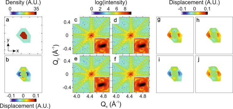
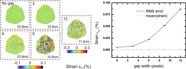
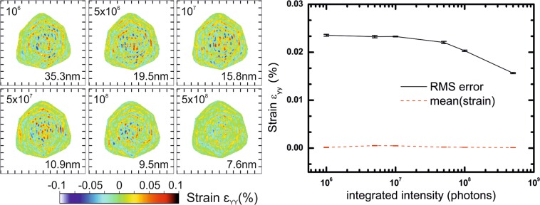
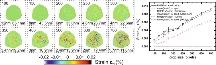
Bragg coherent X-ray diffraction imaging (BCDI) has emerged as a powerful technique to image the local displacement field and strain in nanocrystals, in three dimensions with nanometric spatial resolution. However, BCDI relies on both dataset collection and phase retrieval algorithms that can induce artefacts in the reconstruction. Phase retrieval algorithms are based on the fast Fourier transform (FFT). We demonstrate how to calculate the displacement field inside a nanocrystal from its reconstructed phase depending on the mathematical convention used for the FFT. We use numerical simulations to quantify the influence of experimentally unavoidable detector deficiencies such as blind areas or limited dynamic range as well as post-processing filtering on the reconstruction. We also propose a criterion for the isosurface determination of the object, based on the histogram of the reconstructed modulus. Finally, we study the capability of the phasing algorithm to quantitatively retrieve the surface strain (i.e., the strain of the surface voxels). This work emphasizes many aspects that have been neglected so far in BCDI, which need to be understood for a quantitative analysis of displacement and strain based on this technique. It concludes with the optimization of experimental parameters to improve throughput and to establish BCDI as a reliable 3D nano-imaging technique.

Figure 1

(a) Density (tick spacing corresponds to 25 nm) and (b) displacement u_x of the model used for the simulation. The displacement u_y is fixed to zero. (c) Kinematic sum with positive convention. (d) Kinematic sum with negative convention. This gives the same diffraction pattern as the positive convention. (e) FFT of the complex object calculated using Python. (f) FFT of the complex object with displacement field of opposite sign, calculated using Python. A zoom on the center of the Bragg peak is shown at the bottom right corner. From this we conclude that the correct and unique diffraction pattern corresponding to our complex object is the one in (f) for FFT calculations. (g–j) show the displacement retrieved from diffraction patterns in (c–f) respectively using the Python-based phasing algorithm.

Figure 2

Complex object used for the simulation. (a) Isosurface of the support with 2D slices at the center of the array in (b) XY plane, (c) ZY plane and (d) XZ plane. The support is fixed to 1 inside the crystal and 0 outside. (e) Contour plot of the experimental 3D diffraction pattern of the THH 111 Pt Bragg peak, where the detector gaps are visible. (f–h) Diffraction patterns projected onto XY plane, YZ plane and XZ plane, respectively.

Figure 3

Effect of the cropped size of the FFT window: reconstructions in the XZ plane (Y being the vertical axis). The upper number corresponds to the width of the FFT window in pixels, the bottom left number is the voxel size in nm, and the bottom right number is the resolution obtained from the PRTF. A complex artefact pattern is always present and increases in amplitude when the FFT window is smaller, without affecting strain mean value. Tick spacing corresponds to 50 nm.

Figure 4

Effect of the presence and width of a gap in the detector: reconstructions in the XZ plane (Y being the vertical axis). The numbers displayed in the top left corner correspond to the width of the gap in pixels, and numbers in the bottom right corner to the resolution obtained from the PRTF. Even for a reasonable gap of 4 to 6 pixels, the RMSE of strain artefacts is larger by an order of magnitude compare to the case without gap. When the gap is larger than 9 pixels, the mean strain value starts to deviate from the null value. Tick spacing corresponds to 50 nm.

Figure 5

Effect of the distance between gaps and the central Bragg peak position: reconstructions in the XZ plane (Y being the vertical axis). The numbers displayed in the top left corner correspond to the distance of the gap to the Bragg peak in pixels, and numbers in the bottom right corner to the resolution obtained from the PRTF. From this simulation, we conclude that it is good practice to position the gap as far as possible from the diffracted intensity when measuring a BCDI dataset. Tick spacing corresponds to 50 nm.

Figure 6

Effect of the dynamic range of the data: reconstructions in the XZ plane (Y being the vertical axis). The number in the top left corner corresponds to the total number of photons in the 3D diffraction pattern, and numbers in the bottom right corner to the resolution obtained from the PRTF. In terms of dynamic range, it is equivalent to 1.2 × 10⁴, 6.2 × 10⁴, 1.2 × 10⁵, 6.2 × 10⁵, 1.2 × 10⁶ and 6.2 × 10⁶, respectively. Although a better dynamic range helps for reducing the amplitude of artefacts, it does not compensate the presence of a gap in the detector. Tick spacing corresponds to 50 nm.

Figure 7

Effect of Poisson noise on previous simulation results. Diffraction patterns and reconstructions in the XZ plane (Y being the vertical axis) for a 400 pixels-wide cropping window and 5 × 10⁷ diffracted photons with: (a) no Poisson noise, (b) Poisson noise, (c) no Poisson noise and a detector gap, (d) Poisson noise and a detector gap. Detector gaps are 6 pixels-wide and located 50 pixels away from the Bragg peak. Tick spacing corresponds to 50 nm. Numbers in the bottom right corner correspond to the resolution obtained from the PRTF.

Figure 8

Effect of a single post-phasing apodization step using a Blackman window on the aliasing noise due to the cropped size of the FFT window: reconstructions in the XZ plane (Y being the vertical axis). Only the apodization step has been added to the data processing presented in Fig. 2. The upper number corresponds to the width of the FFT window in pixels, the bottom left number is the voxel size in nm, and the bottom right number is the resolution obtained from the PRTF. Tick spacing corresponds to 50 nm.

Figure 9

Example of phase averaging: reconstructions in the XZ plane (Y being the vertical axis). The numbers displayed in the top left corner correspond to the width in pixels of the 3D averaging window, and numbers in the bottom right corner to the resolution obtained from the PRTF. There is a significant decrease of the RMSE value of strain by one order of magnitude when the averaging window size is similar or larger than the spatial frequency of stripe artefacts. Averaging the phase is a valid approach for this dataset where no high frequency variation is expected in the phase. Tick spacing corresponds to 50 nm.

Figure 10

(a) Reconstructed support volume depending on the isosurface. The red line corresponds to the volume of the model support. (b) Number of voxels in the reconstructed surface layer (in black) which also belong to the model strain surface layer (in red).

Figure 11

(a) Phase model used for the simulation: slice in the XY plane (Y being the vertical axis). (b) Difference of the simulated modulus and the retrieved modulus. (c) Line cut through an edge (at the arrow position in (b)) of simulated and phased modulus. (d) Histogram of the complete 3D modulus distribution and empirical criterion for isosurface level determination. (e) Simulated and (f) retrieved strain ε_YY. (g) Difference between the simulated strain (red) and the retrieved strain (black), with a too low isosurface (32.5%) corresponding to volume conservation. (h) Difference between the simulated strain and the retrieved strain, with an isosurface determined by our criterion (70%). Tick spacing corresponds to 50 nm. The background has been artificially set to grey outside the support.

References

1. Robinson IK, Vartanyants IA, Williams GJ, Pfeifer MA, Pitney JA. Reconstruction of the Shapes of Gold Nanocrystals Using Coherent X-Ray Diffraction. Phys. Rev. Lett. 2001;87:195505. doi: 10.1103/PhysRevLett.87.195505. - DOI - PubMed
1. Robinson IK, Harder R. Coherent X-ray diffraction imaging of strain at the nanoscale. Nat Mater. 2009;8:291–298. doi: 10.1038/nmat2400. - DOI - PubMed
1. Chen-Wiegart YK, Harder R, Dunand DC, McNulty I. Evolution of dealloying induced strain in nanoporous gold crystals. Nanoscale. 2017;9:5686–5693. doi: 10.1039/C6NR09635B. - DOI - PubMed
1. Kim D, et al. Active site localization of methane oxidation on Pt nanocrystals. Nature Communications. 2018;9:3422. doi: 10.1038/s41467-018-05464-2. - DOI - PMC - PubMed
1. Fernández S, et al. In situ structural evolution of single particle model catalysts under ambient pressure reaction conditions. Nanoscale. 2018;11:331–338. doi: 10.1039/C8NR08414A. - DOI - PubMed