The Relationship Between U.S. East Coast Sea Level and the Atlantic Meridional Overturning Circulation: A Review

Abstract

Scientific and societal interest in the relationship between the Atlantic Meridional Overturning Circulation (AMOC) and U.S. East Coast sea level has intensified over the past decade, largely due to (1) projected, and potentially ongoing, enhancement of sea level rise associated with AMOC weakening and (2) the potential for observations of U.S. East Coast sea level to inform reconstructions of North Atlantic circulation and climate. These implications have inspired a wealth of model- and observation-based analyses. Here, we review this research, finding consistent support in numerical models for an antiphase relationship between AMOC strength and dynamic sea level. However, simulations exhibit substantial along-coast and intermodel differences in the amplitude of AMOC-associated dynamic sea level variability. Observational analyses focusing on shorter (generally less than decadal) timescales show robust relationships between some components of the North Atlantic large-scale circulation and coastal sea level variability, but the causal relationships between different observational metrics, AMOC, and sea level are often unclear. We highlight the importance of existing and future research seeking to understand relationships between AMOC and its component currents, the role of ageostrophic processes near the coast, and the interplay of local and remote forcing. Such research will help reconcile the results of different numerical simulations with each other and with observations, inform the physical origins of covariability, and reveal the sensitivity of scaling relationships to forcing, timescale, and model representation. This information will, in turn, provide a more complete characterization of uncertainty in relevant relationships, leading to more robust reconstructions and projections.

Keywords: AMOC; United States; climate model; coastal; review; sea level.

Figure 1

(a) Monthly mean tide gauge sea level (in millimeters relative to year 2000) at the Battery (New York City; blue line). Projections of relative sea level (RSL) change, relative to year 2000, for RCP 2.6 (blue) and RCP 8.5 emission scenarios (red; Kopp et al., 2014). Shading after the year 2000 indicates 17th to 83rd percentile range of RSL projections. (b) Annual mean RSL (in millimeters, with arbitrary offset) measured at 15 U.S. East Coast tide gauges (Holgate et al., 2013) with long and relatively complete records. (c) Linear trend in RSL along the U.S. East Coast from 1900–2017, in millimeters per year, from a Bayesian reconstruction (panel taken from Piecuch, Huybers, et al., 2018).

Figure 2

Schematic of key AMOC‐related components of the North Atlantic Ocean (modified from García‐Ibáñez et al., 2018). Abbreviations are as follows: NRG = Northern Recirculation Gyre; LC = Labrador Current; DWBC = Deep Western Boundary Current; IC = Irminger Current; EGIC = East Greenland‐Irminger Current. Three source waters for North Atlantic Deep Water are noted: LSW = Labrador Sea Water; ISOW = Iceland‐Scotland Overflow Water; DSOW = Denmark Straits Overflow Water. Box indicates the U.S. East Coast region.

Figure 3

The AMOC, averaged over the 1959–2012 period, from a 1/12° resolution model simulation as described in Hughes et al. (2018). The flow is clockwise around positive values, and the stream function is calculated by integrating the southward velocity both zonally and upwards from the bottom. The black contour is at zero.

Figure 4

(a) Change in maximum AMOC strength for a 28 Coupled Model Intercomparison Project Phase 5 model, RCP4.5‐forced, ensemble, from 1976–2000 to 2076–2100, as calculated by Chen et al. (2018). (b) Ensemble mean dynamic sea level change (m) from 1976–2000 to 2076–2100.

Figure 5

Map of the ratio of dynamic sea level change to AMOC change (m/Sv; 2076–2100 minus 1976–2000) for 25 RCP4.5‐forced Coupled Model Intercomparison Project Phase 5 models with AMOC weakening larger than 2 Sv.

Figure 6

(a) From Woodworth et al. (2014). Regression coefficients of annual mean sea level and overturning transport (at the same latitude) for depths between 100 and 1,300 m using a 1° ocean model, for the period 1950–2009, without wind forcing. (b) Linear regression coefficient (α) of DSL change against the change in maximum AMOC strength for the models shown in Figure 5 (m/Sv). (c) Variance in DSL change explained by AMOC change (%). DSL = dynamic sea level; AMOC = Atlantic Meridional Overturning Circulation.

Figure 7

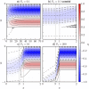
From Wise et al. (2018). Sea level contours (nondimensional; dashed negative) for a given idealized coastal bathymetry along the western boundary of an ocean basin, where x and y are the nondimensional across‐shore and alongshore coordinates, respectively. Vertical dotted lines indicate the continental shelf break at x = S and continental slope floor at x = 1. Panels show sea level patterns for different Péclet numbers: (a) P _a = 0.1, (b) P _a =0.1, (c) P _a =10, and (d) P _a=200. Panels (b)–(d) show only the coastal region.

Figure 8

From Woodworth et al. (2014). (a) Correlations of detrended values of annual mean sea level and overturning transport at the same latitude for depths between 100 and 1,300 m using the simulations shown in Figure 6a (without wind forcing). (b) As in Figure 8a, with winds.

References

1. Andres, M. , Gawarkiewicz, G. G. , & Toole, J. M. (2013). Interannual sea level variability in the western North Atlantic: Regional forcing and remote response. Geophysical Research Letters, 40, 5915–5919. 10.1002/2013GL058013 - DOI
1. Andres, M. , Muglia, M. , Bahr, F. , & Bane, J. (2018). Continuous flow of upper Labrador Sea water around Cape Hatteras. Scientific Reports, 8(1). 10.1038/s41598-018-22758-z - DOI - PMC - PubMed
1. Bakker, P. , Schmittner, A. , Lenaerts, J. T. M. , Abe‐Ouchi, A. , Bi, D. , van den Broeke, M. R. , Chan, W. L. , Hu, A. , Beadling, R. L. , Marsland, S. J. , Mernild, S. H. , Saenko, O. A. , Swingedouw, D. , Sullivan, A. , & Yin, J. (2016). Fate of the Atlantic Meridional Overturning Circulation: Strong decline under continued warming and Greenland melting. Geophysical Research Letters, 43, 12,252–12,260. 10.1002/2016GL070457 - DOI
1. Beadling, R. L. , Russell, J. L. , Stouffer, R. J. , & Goodman, P. J. (2018). Evaluation of subtropical North Atlantic Ocean circulation in CMIP5 models against the observational array at 26.5°N and its changes under continued warming. Journal of Climate. 10.1175/JCLI-D-17-0845.1 - DOI
1. Becker, J. M. , & Salmon, R. (1997). Eddy formation on a continental slope. Journal of Marine Research, 55(2), 181–200. 10.1357/0022240973224418 - DOI
LinkOut - more resources