. 2019 Dec;22(12):2040-2049.
doi: 10.1038/s41593-019-0533-x. Epub 2019 Nov 25.

Unsupervised identification of the internal states that shape natural behavior

Affiliations

Unsupervised identification of the internal states that shape natural behavior

Adam J Calhoun et al. Nat Neurosci. 2019 Dec.

Erratum in

Abstract

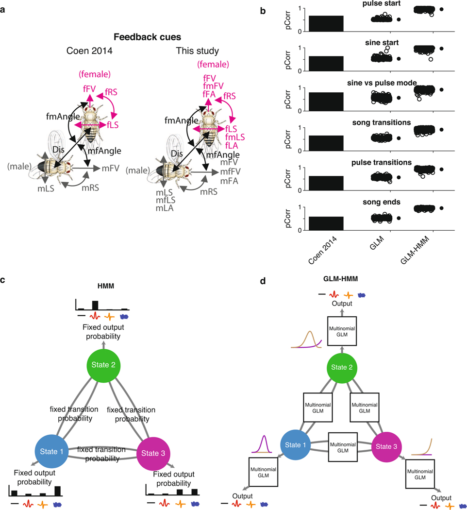
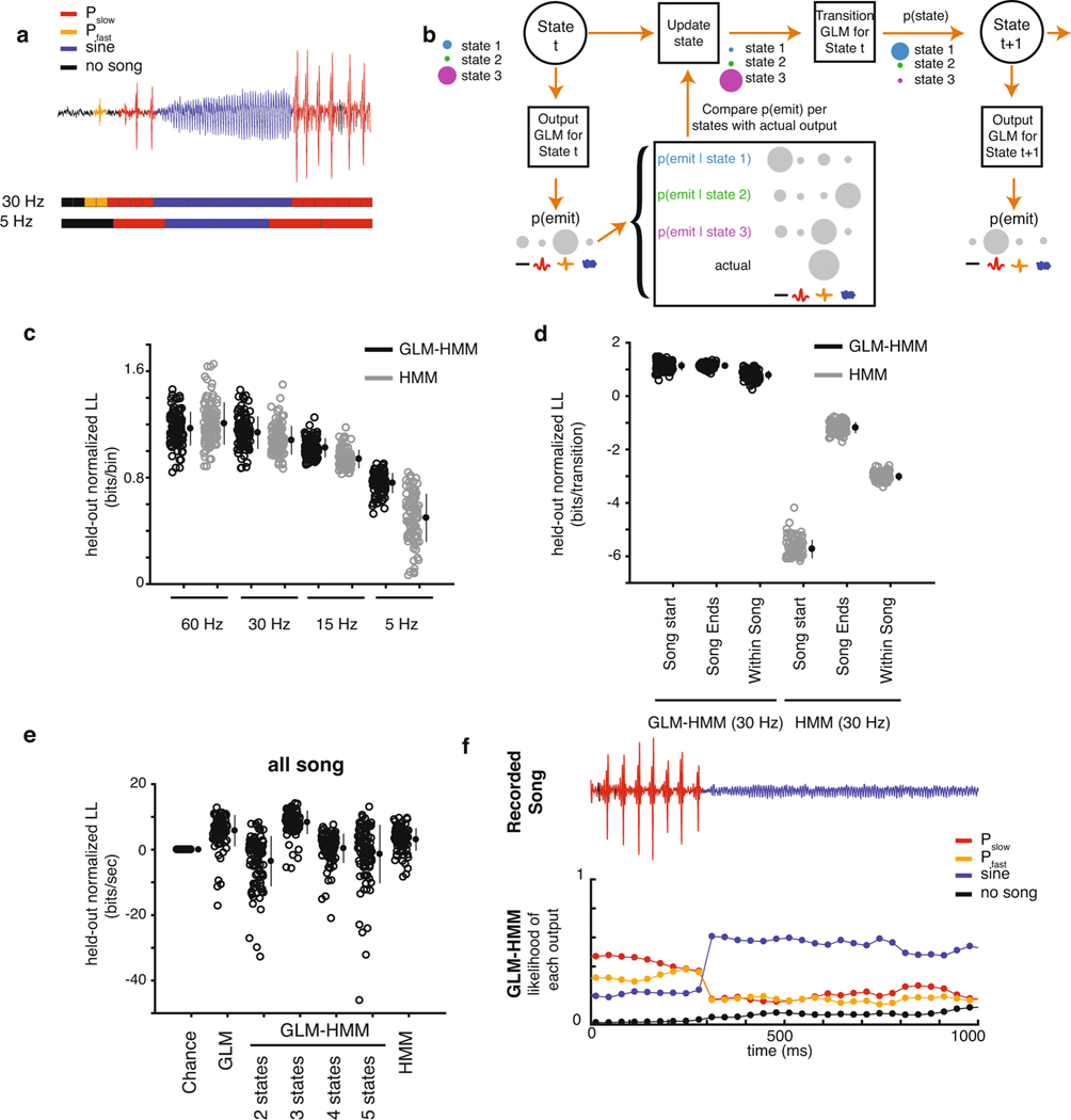
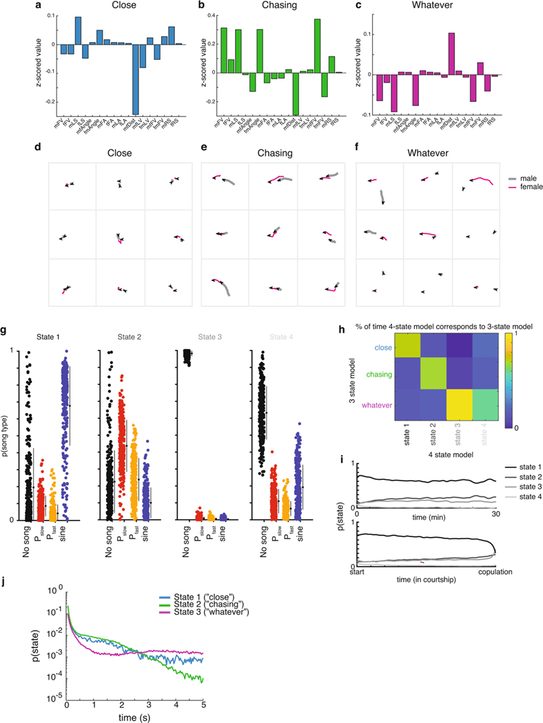
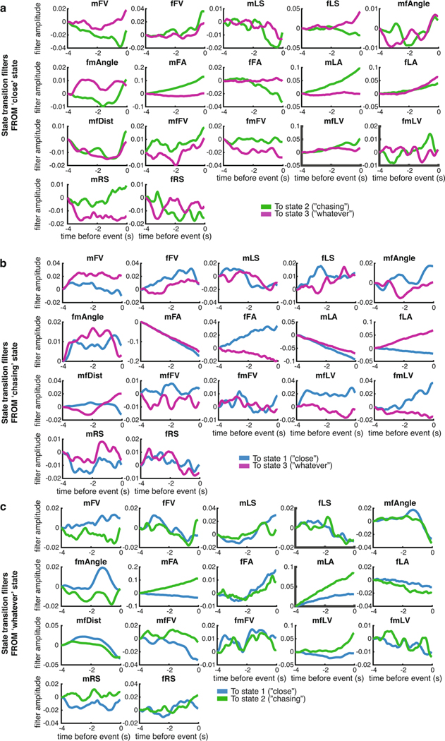
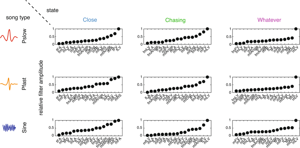
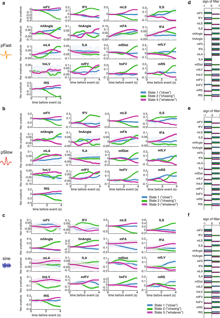
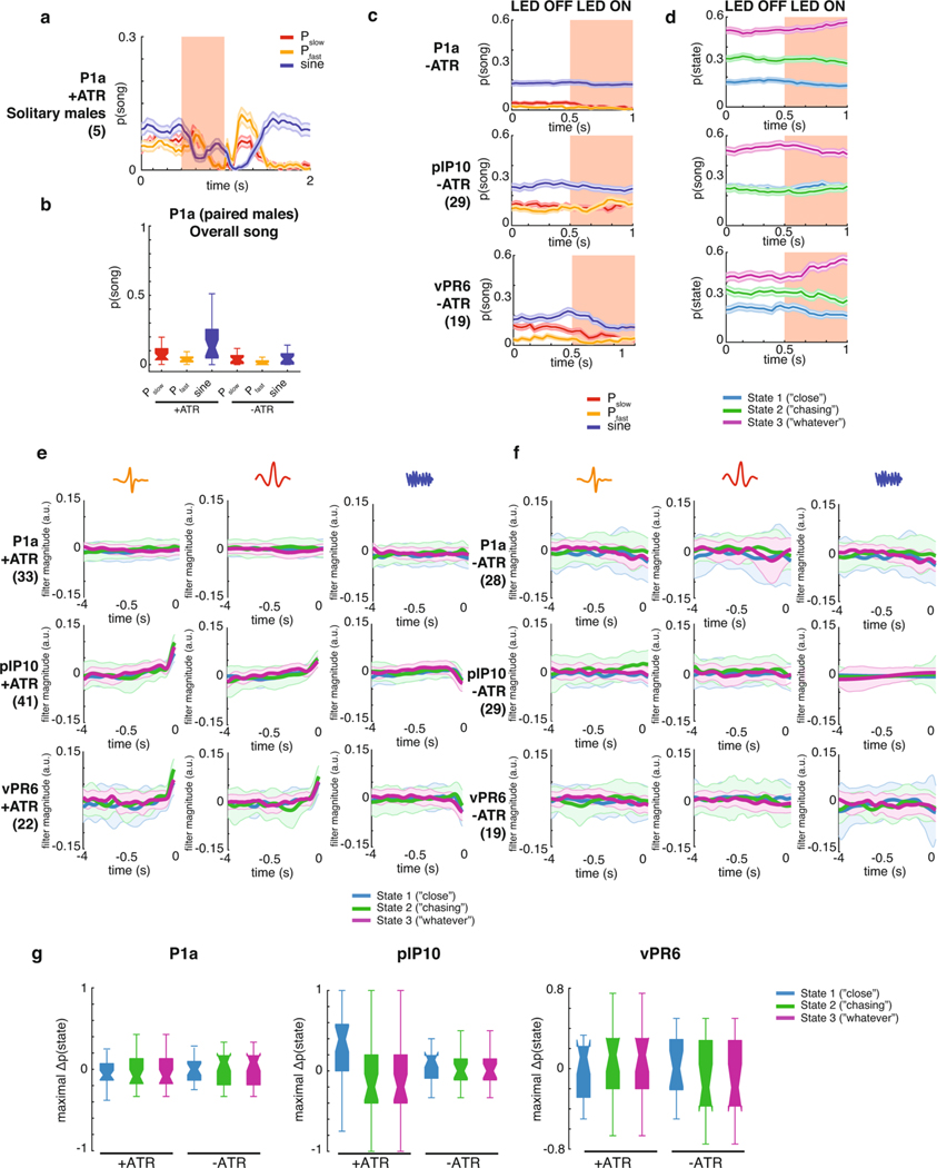
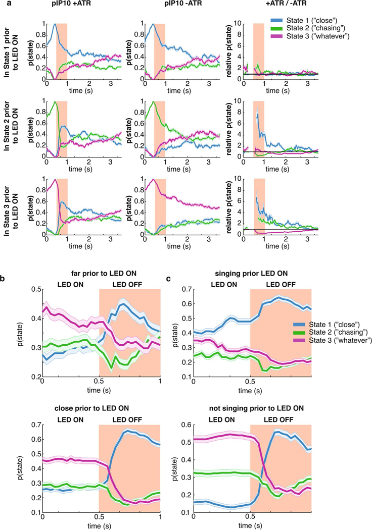
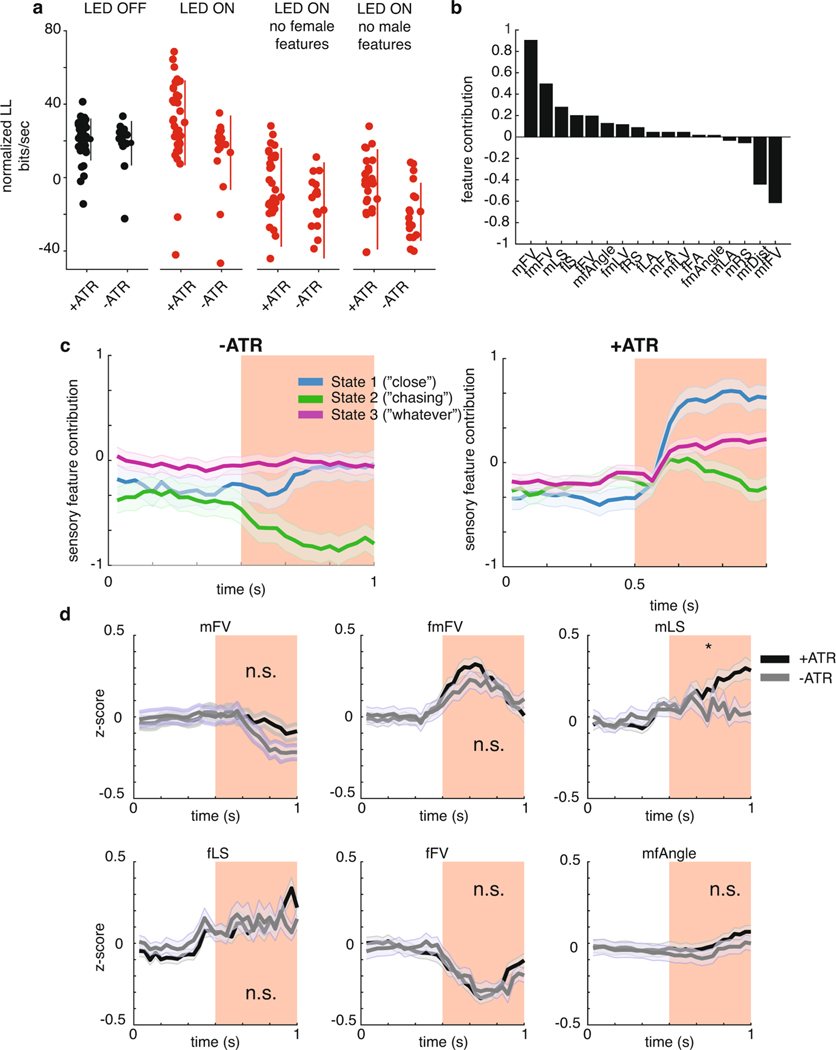
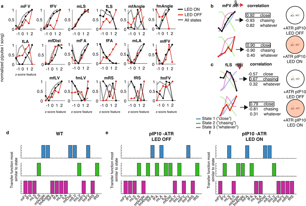
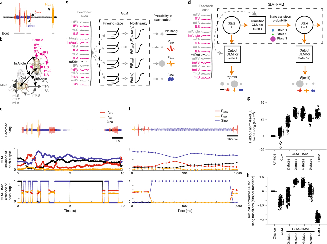
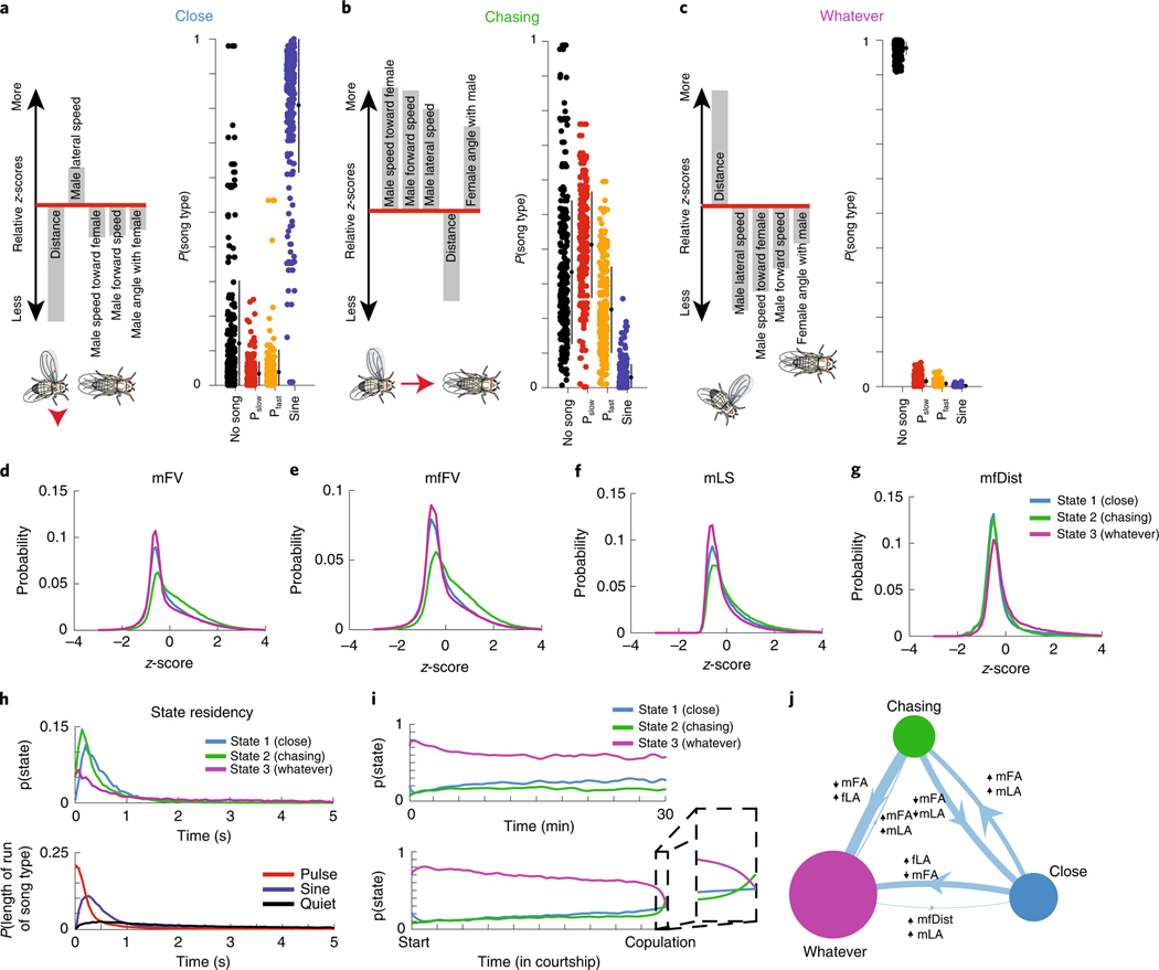
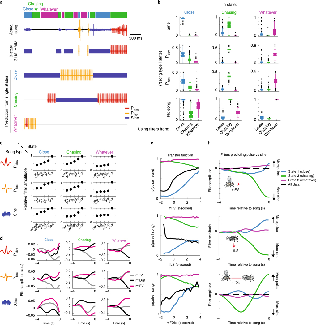
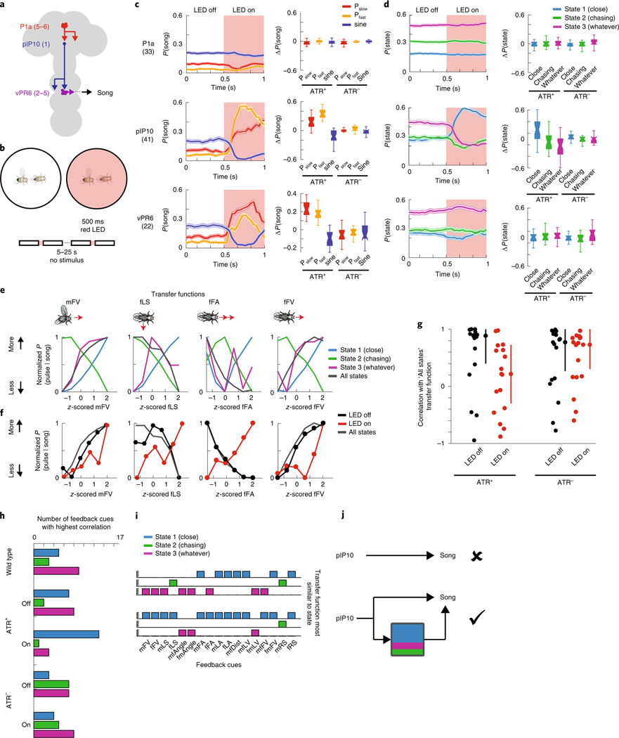
Internal states shape stimulus responses and decision-making, but we lack methods to identify them. To address this gap, we developed an unsupervised method to identify internal states from behavioral data and applied it to a dynamic social interaction. During courtship, Drosophila melanogaster males pattern their songs using feedback cues from their partner. Our model uncovers three latent states underlying this behavior and is able to predict moment-to-moment variation in song-patterning decisions. These states correspond to different sensorimotor strategies, each of which is characterized by different mappings from feedback cues to song modes. We show that a pair of neurons previously thought to be command neurons for song production are sufficient to drive switching between states. Our results reveal how animals compose behavior from previously unidentified internal states, which is a necessary step for quantitative descriptions of animal behavior that link environmental cues, internal needs, neuronal activity and motor outputs.


Conflict of interest statement

Competing interests

The authors declare no competing interests.

Figures

Extended Data Fig. 1 |
Extended Data Fig. 1 |. Comparison of GLMs and GLM-HMM.
a, Fly feedback cues used for prediction in (Coen et al. 2014) (left) or the current study (right). b, Comparison of model performance using probability correct (‘pCorr’) (see Methods) for predictions from (Coen et al. 2014) (reproduced from that paper) for the single-state GLM (See Fig. 1c) and 3-state GLM-HMM (see Fig. 1d). Each open circle represents predictions from one courtship pair. The same pairs were used when calculating the pCorr value for each condition (GLM and 3-state GLM-HMM); filled circles represent mean +/− SD; 100 shown for visualization purposes. c, Schematic of standard HMM, which has fixed transition and emission probabilities. d, Schematic of GLM-HMM in the same format, with static probabilities replaced by dynamic ones. Example filters from the GLM are indicated with the purple and light brown lines.
Extended Data Fig. 2 |
Extended Data Fig. 2 |. Assessing model predictions.
a, Illustration of how song is binned for model predictions. Song traces (top) are discretized by identifying the most common type of song in between two moments in time, allowing for either fine (middle) or coarse (bottom) binning - see Methods. b, Illustration of how model performance is estimated, using one step forward predictions (see Methods). c, 3-state GLM-HMM performance at predicting each bin (measured in bits/bin) when song is discretized or binned at different frequencies (60 Hz, 30 Hz, 15 Hz, 5 Hz) and compared to a static HMM - all values normalized to a ‘chance’ model (see Methods). Each open circle represents predictions from one courtship pair. Note that the performance at 30Hz represents a re-scaled version of the performance shown in Fig. 1g. Filled circles represent mean +/− SD, n=100. d, Comparison of the 3-state GLM-HMM with a static HMM for specific types of transitions when song is sampled at 30 Hz (in bits/transition, equivalent to bits/bin; compare with panel (c)) - all values normalized to a ‘Chance’ model (see Methods). The HMM is worse than the ‘Chance’ model at predicting transitions. Filled circles represent mean +/− SD, n=100. e, Performance of models when the underlying states used for prediction are estimated ignoring past song mode history (see b) and only using the the GLM filters - all values normalized to a ‘Chance’ model (see Methods). The 3-state GLM-HMM significantly improves prediction over ‘Chance’ (p = 6.8 e-32, Mann-Whitney U-test) and outperforms all other models. Filled circles represent mean +/− SD, n=100. f, Example output of GLM-HMM model when the underlying states are generated purely from feedback cues (e).
Extended Data Fig. 3 |
Extended Data Fig. 3 |. Evaluating the states of the GLM-HMM.
a-c. The mean value for each feedback cue in the (a) ‘close’, (b) ‘chasing’, or (c) ‘whatever’ state (see Methods for details on z-scoring). d-f. Representative traces of male and female movement trajectories in each state. Male trajectories are in gray and female trajectories in magenta. Arrows indicate fly orientation at the end of 660 ms. g. In the 4-state GLM-HMM model, the probability of observing each type of song when the animal is in that state. Filled circles represent individual animals (n=276 animals, small black circles with lines are mean +/− SD). h. The correspondence between the 3-state GLM-HMM and the 4-state GLM-HMM. Shown is the conditional probability of the 3-state model being in the ‘close’, ‘chasing’, or ‘whatever’ states given the state of the 4-state model. i. The mean probability across flies of being in each state of the 4-state model when aligned to absolute time (top) or the time of copulation (bottom). j. Probability of state dwell times generated from feedback cues. These show non-exponential dwell times on a y-log plot.
Extended Data Fig. 4 |
Extended Data Fig. 4 |. State transition filters.
a-c, State-transition filters that predict transitions from one state to another for each feedback cue (see Fig. 1B for list of all 17 feedback cues used in this study).
Extended Data Fig. 5 |
Extended Data Fig. 5 |. Amplitude of output filters.
The amplitude of output filters (see Methods) for each state/output pair. Output filter amplitudes were normalized between 0 (smallest filter amplitude) and 1 (largest filter amplitude).
Extended Data Fig. 6 |
Extended Data Fig. 6 |. Output filters.
a-c, Output filters for each feedback cue (see Fig. 1b) that predict the emission of each song type for a given state. ‘No song’ filters are not shown as these are fixed to be constant, and song type filters are in relation to these values (see Methods). Heavy line represents mean, shading represents Sem. d-e, Sign of filter for each emission filter shows the same feature can be excitatory or inhibitory depending on the state.
Extended Data Fig. 7 |
Extended Data Fig. 7 |. Activation of song pathway neurons.
a, Solitary ATR-fed P1a males produce song when exposed to the same LED stimulus used in Figure 4. In solitary males, song production is both long-lasting and time-locked to the LED stimulus. Number of animals in parentheses (n=5), heavy line represents mean, shading represents SEM. b, ATR-fed P1a males courting a female produce significantly more Pfast (p = 1e-4), Pslow (p = 1e-3), and significantly-different amounts of sine song (p = 0.009). All p-values from Mann-Whitney U-test. Animals from (a) (n=5), center lines of box plots represent median, the bottom and top edges represent the 25th and 75th percentiles (respectively). Whiskers extend to +/− 2.7 times the standard deviation. c, The probability of observing each song mode aligned to the opto stimulus shows that LED activation of flies not fed ATR does not increase song production. Number of animals in parentheses, heavy line represents mean, shading represents SEM. d, The probability of the model being in each state aligned to the opto stimulus shows that LED activation of flies not fed ATR does not change state residence. Error bars represent Sem. Number of animals in parentheses, heavy line represents mean, shading represents SEM. e-f, ‘Opto’ filters represent the contribution of the LED to the production of each type of song for (e) ATR+ and (f) ATR− flies. Number of animals in parentheses, heavy line represents mean, shading represents SEM. The filters for each strain and song type are not significantly different between states. g, Measuring the maximal change in state probability between LED ON and LED OFF shows that only pIP10 activation produces a significant difference between ATR+ and ATR− flies (two-tailed t test). Number of animals in parentheses in (e-f), center lines of box plots represent median, the bottom and top edges represent the 25th and 75th percentiles (respectively). Whiskers extend to +/− 2.7 times the standard deviation. All p-values from two-tailed t test.
Extended Data Fig. 8 |
Extended Data Fig. 8 |. Activating piP10 biases males toward the close state.
a, Conditioning on which state the animal is in prior to the light being on (left, ATR-fed pIP10 flies, n=41; middle ATR-free pIP10 flies, n=28; right, ratio of ATR-fed to ATR-free state dwell time), activation of pIP10 results in an increase in the probability of being in the close state unless the animal was already in the close state. Shaded area is SRM. b, When the male was both close (<5mm) and far (> 8mm), pIP10 activation increases the probability that the animal will enter the close state. Shaded area is SRM. c. When the male was already either singing or not singing, pIP10 activation increases the probability that the animal will enter the close state. Shaded area is SRM.
Extended Data Fig. 9 |
Extended Data Fig. 9 |. Bias toward close state is due to the altered use of feedback cues.
a, Predictive performance is not significantly different between light ON and light OFF conditions for both ATR-fed (n=41, p=0.08) and ATR-free animals (n=28, p=0.46). Performance suffers without male (+ATR p=4e-12, −ATR p=1e-9) or female feedback cues (+ATR p=1e-10, −ATR p=1e-9), suggesting these state-specific features are needed to predict animal behavior. Dots represent individual flies, center line is mean and lines are +/− SD. All statistical tests are Mann-Whitney U-test. b, The similarity between each feedback cue and the filters for the ‘close’ state are subtracted by the similarity of that feedback cue to the filters for the ‘chasing’ state during LED activation of ATR-fed pIP10 flies. This reveals song patterning is more similar to the ‘close’ state than the ‘chasing’ state for most feedback cues. c, Animals that were not fed ATR (n=28) do not show a change in the contribution of the feedback cues to being in a given state, while animals that are fed ATR (n=41) do show a change in feedback cue contribution. Shaded area is SRM. d, Most aspects of the animal trajectory do not differ in response to red light when males are either fed (black, n=41) or not fed (gray, n=28) ATR food. Plotted are the six strongest contributors from (b). p-values are p=0.056 for mFV, p=0.11 for fmFV, 9.7e-5 for mLS, p=0.64 for fLS, p=0.67 for fFV, p=0.009 for mfAngle Mann-Whitney U-test, significance at p = 0.05 corrected to p = 0.0083 by Bonferroni. * represents p < 0.0083, n.s. p > 0.008. Shaded area is SEM.
Extended Data Fig. 10 |
Extended Data Fig. 10 |. The relationship between feedback cues and song patterns changes when LED is ON in piP10 +ATR flies.
a, The transfer functions of each feedback cue when the LED is OFF (black) and when the LED is ON (red) compared to the wild-type average (dark gray). b-c, Illustration of Pearson’s correlation between transfer functions of two feedback cues (mFV (g) and fLS (h)) when the LED is off (top, black) and on (bottom, red) and the transfer function in each state (not the average as in Fig. 4f). The feature is considered most similar to the state with which it has the highest Pearson’s correlation. All ATR-fed pIP10 animals were used (n=41). d, The state transfer function that is closest to the wild-type average for each feedback cue. For instance, the mFV average is closest to the ‘whatever’ state and the fLS average is closest to the ‘chasing’ state. e-f, Same as (d), but for pIP10 – ATR flies when the LED is off (e) or on (f).
Fig. 1 |
Fig. 1 |. A model with hidden states effectively predicts song patterning.
a, The fly song modes analyzed: no song (black), Pfast (orange), Pslow (red) and sine (blue). Song is organized into trains of a particular type of song in a sequence (multiple pulses in a row constitute a pulse train) as well as bouts (multiple trains followed by no song, represented here by a black line). b, The fly feedback cues analyzed: mFV and female forward velocity (fFV); male lateral speed (mLS), fLS, male rotational speed (mRS) and female rotational speed (fRS); male forward lateral accelerations (mFA), female forward accelerations (fFA), male lateral accelerations (mLA) and female lateral accelerations (fLA); the component of male forward and lateral velocity in the direction of the female (mfFV and mfLS) and the component of the female forward and lateral velocity in the direction of the male (fmFV and fmLS); the distance between the animals (mfDist) and the absolute angle from female/male heading to male/female center (mfAngle and fmAngle). c, Schematic illustrating the multinomial GLM, which takes feedback cues as input and passes these cues through a linear filtering stage. There is a separate set of linear filters for each possible song mode. These filters are passed through a nonlinearity step, and the relative probability of observing each output (no song, Pfast, Pslow, sine song) gives the overall likelihood of song production. d, Schematic illustrating the GLM–HMM. At each time point t, the model is in a discrete hidden state. Each hidden state has a distinct set of multinomial GLMs that predict the type of song that is emitted, as well as the probability of transitioning to a new state. e, Top: 10 s of natural courtship song consisting of no song (black), Pfast, Pslow and sine. Middle: the conditional probability of each output type for this stretch of song under the standard GLM. Bottom: the conditional probability of the same song data under the three-state GLM–HMM; predictions are made one step forward at a time using past feedback cues and song mode history (see Methods). f, Top: 100 ms of natural song. Middle and bottom: conditional probability of each song mode under GLM (middle) and GLM–HMM (bottom), as in e. g, Normalized log-likelihood (LL) on test data (in bits s−1; see methods). The GLM outperforms the chance model (P = 2.9 × 10⁻²⁹), but the three-state GLM–HMM produces the best performance (each open circle represents predictions from one courtship pair (only 100 of the 276 pairs shown for visual clarity); filled circles represent the mean ± s.d.). The three-state model outperformed a two-state GLM–HMM (P = 2.2 × 10⁻³³) and a five-state GLM–HMM (P = 4.1 × 10⁻³⁰), but was not significantly different from a four-state model (P = 0.16). On the basis of this same metric, the three-state GLM–HMM slightly outperformed a Hmm (1 bit s−1 improvement, P = 1.8 × 10⁻⁵). All P values from Mann–Whitney U-tests. h, Normalized test log-likelihood during transitions between song modes (for example, transition from sine to Pslow). The three-state GLM–HMM outperformed the GLM (P ≤ 2.55 × 10⁻³⁴) and the two-state GLM–HMM (P = 2.3 × 10⁻³⁴), and substantially outperformed the Hmm (P ≤ 2.55 × 10⁻³⁴). Filled circles represent the mean ± s.d., 100 of the 276 pairs shown. All P values from Mann–Whitney U-tests.
Fig. 2 |
Fig. 2 |. Three sensorimotor strategies.
ac, Left: the five feedback cues that are most different from the mean when the animal is in the Close (a), Chasing (b) or Whatever (c) state (see Methods for details on z-scoring). Illustration of flies is a representation of each state according to these feedback cues. Right: the probability of observing each type of song when the animal is in that state. Filled circles represent individual animals (n = 276 animals, small black circles with lines are the mean ± s.d.). dg, Distributions of values (z-scored, see Methods) for four of the feedback cues (see Fig. 1b) and for each state. Although a state may have features that are larger or smaller than average, the distributions are highly overlapping (the key in g also applies to df). h, Top: the dwell times of the Close, Chasing and Whatever states across all of the data (including both training and validation sets). Bottom: the dwell times of sine trains, pulse trains and stretches of no song (see Fig. 1a for definition of song modes; Pfast and Pslow are grouped together here) across all of the data are dissimilar from the dwell times of the states with which they are most associated. Data from all 276 animals. i, Top: the mean probability across flies of being in each state fluctuated only slightly over time when aligned to absolute time (bottom) or the time of copulation (bottom). Immediately before copulation, there was a slight increased probability of being in the Chasing state (bottom, zoomed-in area). Data are from all 276 animals. j, Areas of circles represent the mean probability of being in each state and the width of each line represents the fixed probability of transitioning from one state to another. The filters that best predicted transitioning between states (and modify the transition probabilities) label each line, with the up arrow representing feedback cues that increase the probability and the down arrow representing feedback cues that decrease the probability.
Fig. 3 |
Fig. 3 |. Internal states are defined by distinct mappings between feedback cues and song behavior.
a, A stretch of 500 ms of song production from the natural courtship dataset, with the prediction of states indicated above in colored squares. The prediction of the full GLM–HMM model (third row) is very different from the prediction if we assume that the animal is always in the Close state, Chasing state or Whatever state. The output using the song prediction filters from only that state is illustrated in the lower three rows. b, The conditional probability (across all data, n = 276 animals, error bars represent the s.e.m.) of observing a song mode in each state (predicted by the full three-state GLM–HMM), but using output filters from only one of the states. Conditional probability of the appropriate state is larger than the conditional probability of the out-of-state prediction (largest P = 6.7 × 10⁻⁶ across all comparisons, mann–Whitney U-test). Song-mode predictions were highest when using output filters from the correct state. Center lines of box plots represent the median, the bottom and top edges represent the 25th and 75th percentiles, respectively. Whiskers extend to ±2.7 times the standard deviation. c, The five most predictive output filters for each state and for prediction of each of the three of the types of song. Filters for types of song are relative to no-song filters, which are set to a constant term (see Methods). d, Example output filters for each state revealed that even for the same feedback cues, the GLM–HMM shows distinct patterns of integration. Plotted here are the mFV, mfDist and the mfFV; filters can change sign and shape between states. e, Transfer functions (the conditional probability of observing song choice (y axis) as a function of the magnitude of each feedback cue (x axis)) for producing pulse (both Pslow and Pfast) versus sine have distinct patterns based on state. For mFV (upper), fLS (middle) and mfDist (lower), the average relationship or transfer function between song choice and the movement cue (black line) differs with transfer functions separated by state (blue, green and purple). f, Output filters that predict pulse versus sine song for each of the following three feedback cues: mFV (upper), fLS (middle) and mfDist (lower).
Fig. 4 |
Fig. 4 |. Optogenetic activation of song pathway neurons and state switching.
a, Schematic of the three classes of neurons in the Drosophila song-production pathway. b, Protocol for optogenetically activating song-pathway neurons using csChrimson targeted to each of the neuron types in a. c, Left: the observed probability of each song mode aligned to the onset of the optogenetic stimulus. Right: the difference between the mean during LED on from the mean during LED off before stimulation. The numbers of flies tested are indicated in parentheses; error bars represent the s.e.m. Control males are of the same genotype but have not been fed ATR, the required co-factor for csChrimson. Center lines of box plots represent the median, the bottom and top edges represent the 25th and 75th percentiles, respectively. Whiskers extend to ±2.7 times the standard deviation. d, Left: the posterior probability of each state given the feedback cues and observed song (under the three-state GLM–HMM trained on wild-type data), aligned to the onset of optogenetic stimulation; error bars are the s.e.m. Right: activation of pIP10 neurons biases males to the close state and away from the Chasing and Whatever states. The difference between the mean during LED on from the mean during LED off before stimulation is shown on the right. The numbers of flies are listed in parentheses in c. Center lines of box plots represent the median, while the bottom and top edges represent the 25th and 75th percentiles, respectively. Whiskers extend to ±2.7 times the standard deviation. e, Comparison of transfer functions (the conditional probability of observing song choice (y axis) as a function of the magnitude of each feedback cue (x axis; see also Fig. 3e). Shown here are transfer functions for four feedback cues (mFV, fLS, fFA and fFV). Average across all states (dark gray) represents the transfer function from all data without regard to the state assigned by the model. Transfer functions are calculated from all data. f, Transfer functions for the same four feedback cues shown in e, but in animals expressing csChrimson in pIP10 while the LED is off (black) or on (red); transfer functions for data from wild-type animals across all states (dark gray) reproduced from e. g, For all 17 feedback cues, median Pearson’s correlation between transfer functions between all states and the four conditions (pIP10 and ATR+ (LED off or on) or ATR (LED off or on). Error bars represent the median absolute deviation. h, The number of feedback cues with the highest correlation between the wild-type transfer functions (separated by state) and the transfer functions for each of the conditions (pIP10 and ATR+ (LED off or on) and pIP10 and ATR (LED off or on). Blue represents transfer functions most similar to the Close state, green to the Chasing state, and purple to the Whatever state. i, Unpacking the data in h for the ATR+ condition. j, Top: schematic of the previous view of pIP10 neuron function. Bottom: pIP10 activation both drives song production and state switching; this revised view of pIP10 neuron function would not have been possible without the computational model.

Comment in

Similar articles

Cited by

References

    1. Berman GJ Measuring behavior across scales. BMC Biol. 16, 23 (2018). - PMC - PubMed
    1. Calhoun AJ & Murthy M. Quantifying behavior to solve sensorimotor transformations: advances from worms and flies. Curr. Opin. Neurobiol 46, 90–98 (2017). - PMC - PubMed
    1. Egnor SER & Branson K. Computational analysis of behavior. Annu. Rev. Neurosci 39, 217–236 (2016). - PubMed
    1. Anderson DJ Circuit modules linking internal states and social behaviour in flies and mice. Nat. Rev. Neurosci 17, 692–704 (2016). - PubMed
    1. Stringer C. et al. Spontaneous behaviors drive multidimensional, brain-wide activity. Science 364, eaav7893 (2019). - PMC - PubMed

Publication types