Chromatin structure dynamics during the mitosis-to-G1 phase transition

Abstract

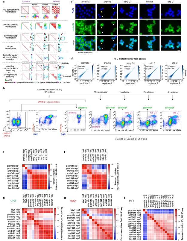
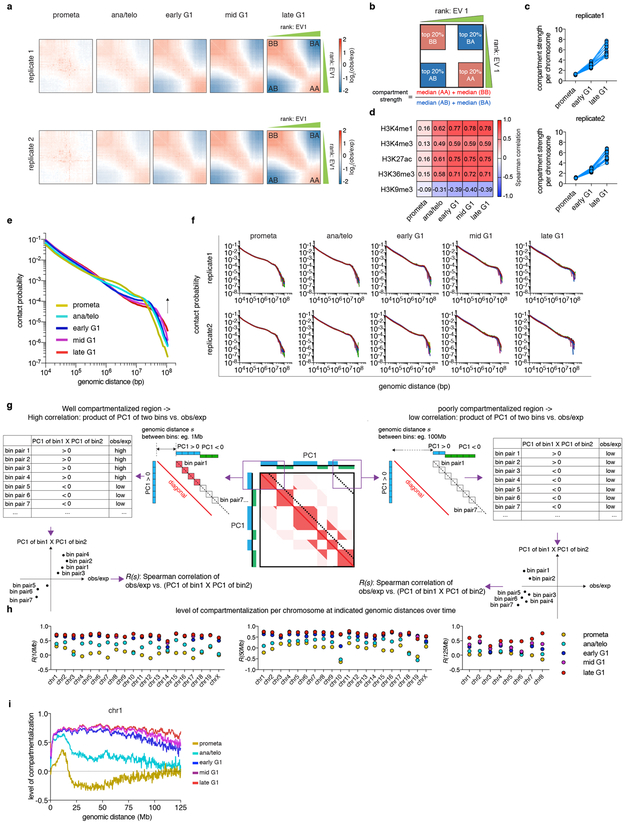
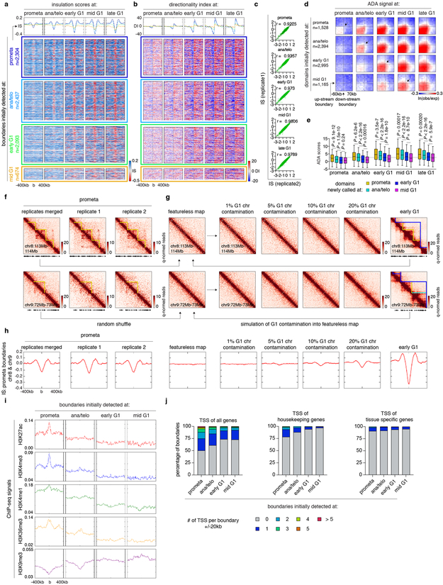
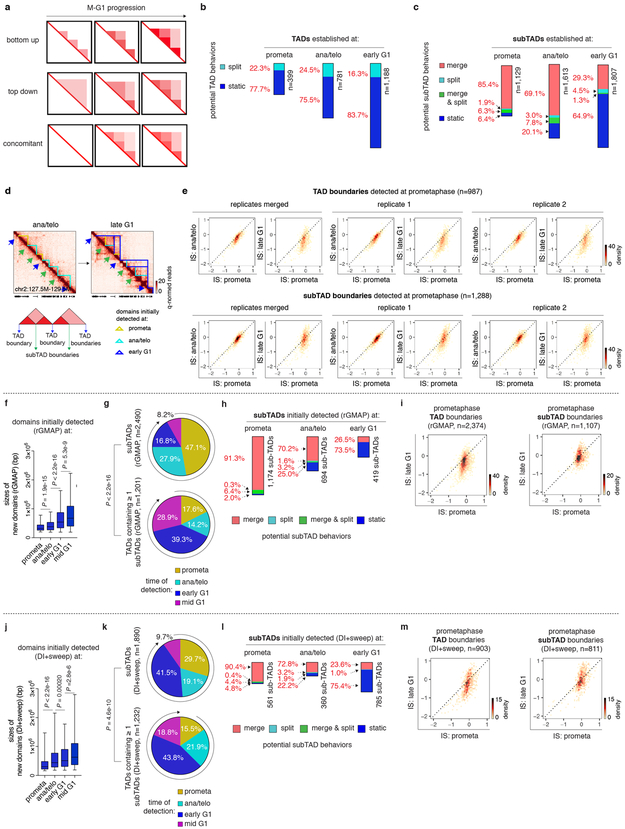
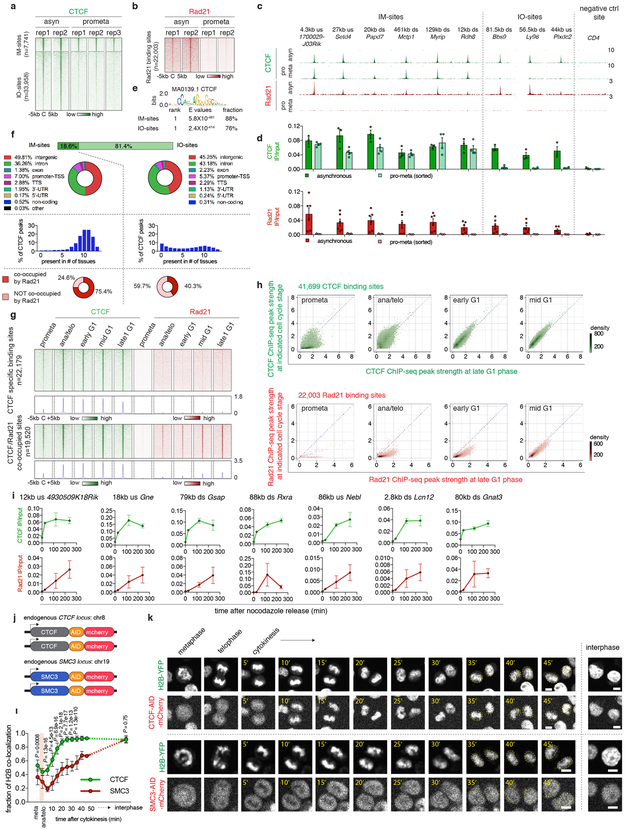
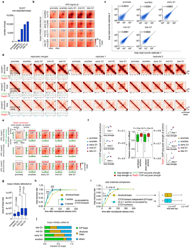
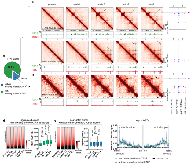
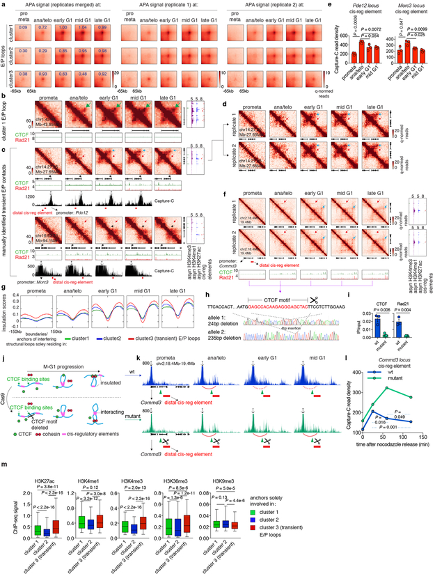
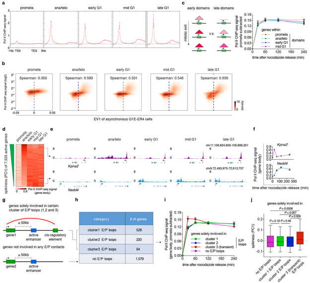
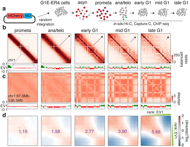
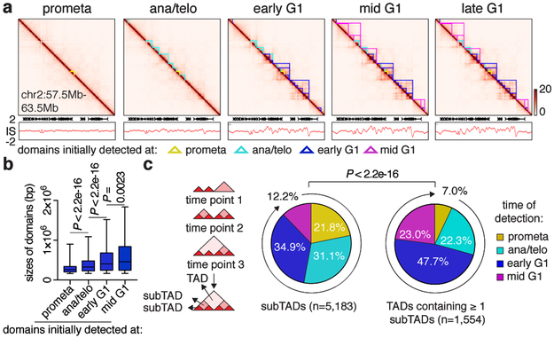
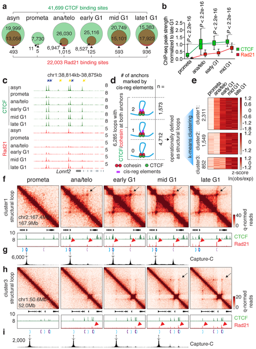
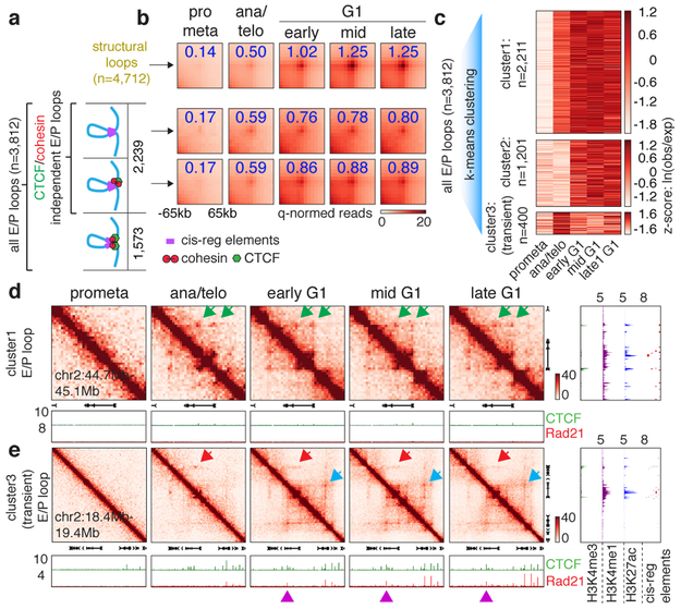
Features of higher-order chromatin organization-such as A/B compartments, topologically associating domains and chromatin loops-are temporarily disrupted during mitosis^1,2. Because these structures are thought to influence gene regulation, it is important to understand how they are re-established after mitosis. Here we examine the dynamics of chromosome reorganization by Hi-C after mitosis in highly purified, synchronous mouse erythroid cell populations. We observed rapid establishment of A/B compartments, followed by their gradual intensification and expansion. Contact domains form from the 'bottom up'-smaller subTADs are formed initially, followed by convergence into multi-domain TAD structures. CTCF is partially retained on mitotic chromosomes and immediately resumes full binding in ana/telophase. By contrast, cohesin is completely evicted from mitotic chromosomes and regains focal binding at a slower rate. The formation of CTCF/cohesin co-anchored structural loops follows the kinetics of cohesin positioning. Stripe-shaped contact patterns-anchored by CTCF-grow in length, which is consistent with a loop-extrusion process after mitosis. Interactions between cis-regulatory elements can form rapidly, with rates exceeding those of CTCF/cohesin-anchored contacts. Notably, we identified a group of rapidly emerging transient contacts between cis-regulatory elements in ana/telophase that are dissolved upon G1 entry, co-incident with the establishment of inner boundaries or nearby interfering chromatin loops. We also describe the relationship between transcription reactivation and architectural features. Our findings indicate that distinct but mutually influential forces drive post-mitotic chromatin reconfiguration.

Extended Data Figure 1 ∣. Models, experimental workflow and data quality control.

a, 1^st panel: Schematic illustration of the early emergence, gradual intensification and expansion of A/B compartments (checkerboards) from prometaphase to late G1 phase, coupled with schematics of chromatin organization. 2^nd panel: SubTADs (small triangles) emerge first after mitotic exit, followed by convergence into a TAD (big triangle). 3^rd panel: Formation of a structural loop coincides with the positioning of cohesin, but not CTCF after mitosis. 4^th panel: The gradual extrusion of cohesin complex along DNA fiber from one anchor point with CTCF, reflected as enrichment of interactions between the anchor and a continuum of DNA loci on the contact map. 5^th panel: Fast formation of E/P loops after mitosis. 6^th panel: The interplay between transient E/P loops and boundaries or structural loops. b, Experimental workflow: representative flow cytometry plots showing the nocodazole arrest/release strategy based on pMPM2 (prometaphase), mCherry-MD signal, and DNA content (DAPI) staining. Similar observations were made in > 5 independent experiments. c, Representative images showing DAPI and lamin B1 staining of FACS purified cells across all cell cycle stages. Similar observations were made in 2 independent experiments. The mitotic index of prometaphase cells after FACS purification is on average > 98%. Yellow and white arrowheads indicate anaphase and telophase cells respectively. Scale bar: 10μm. d, Hexbin plots showing the high correlation of Hi-C raw read counts between two biological replicates across all cell cycle stages. Bin size: 250kb. e, Heatmap showing the Pearson correlation among all Hi-C samples, based on the eigenvector 1 of 250kb bins. f, Heatmap showing the Pearson correlation among all Hi-C samples based on raw read counts. Bin size: 250kb. (g-i), Heatmaps showing Pearson correlation of CTCF, Rad21 and Pol II ChIP-seq among all samples, respectively. Note the overall high replicate concordance with low correlation coefficients among replicates only observed in samples with low signal/noise ratios, e.g. in prometaphase.

Extended Data Figure 2 ∣. Compartment strengthening and expansion from ana/telophase throughout late G1.

a, Saddle plots showing the progressive gain of compartment strength over time in two biological replicates. b, Schematic showing the calculation of compartment strength. c, Line graphs showing the progressive increase of compartment strength of each individual chromosome (represented by dots) in two biological replicates. d, Heatmap showing the genome wide Spearman correlation coefficients between eigenvector 1 values and asynchronous cell derived ChIP-seq signals for the indicated histone marks. e, Chromosome averaged distance dependent contact frequency P(s) plots at all cell cycle stages. f, P(s) plots of each individual chromosome of two biological replicates. g, A schematic illustrating how compartmentalization levels R(s) were calculated at different distance scales (e.g. 1Mb or 100Mb). Each dotted line indicates a series of 250kb bin-bin pairs that are separated by a given genomic distance s (the distance from the diagonal to the dotted line). For all bin-bin pairs separated by distance of s, a Spearman correlation coefficient R(s) was generated between obs/exp and the product of two eigenvector 1 values (PC1 (bin1) × PC1 (bin2)). R(s) is expected to be high in well compartmentalized regions (left panel) and low at large distance scales with no compartments (right panel). h, Replicate averaged R(s) of each individual chromosome across all cell cycle stages when s equals to 10, 50 and 125Mb (only eight chromosomes computed at this distance scale). i, Line graph showing the level of compartmentalization of chr1 against genomic distance at each cell cycle stage.

Extended Data Figure 3 ∣. Domain detection and residual “domain-like” structures in prometaphase.

(a-b), Meta-region plots and density heatmaps of insulation scores and directionality index centered around domain boundaries initially detected at each cell cycle stage. c, Scatter plots showing Pearson correlations of insulation scores at domain boundaries between two biological replicates. d, Aggregated domain analysis (ADA) of domains initially detected at each cell cycle stage. e, Box plots showing ADA scores over time of domains initially detected at prometa (n=1,360), ana/telo (n=2,260), early G1 (n=2,875) and mid G1 (n=1,112). For all box plots, center lines denote medians; box limits denote 25-75 percentile; whiskers denote 5-95 percentile. P values were calculated from two-sided Mann-Whitney U test. Dotted line indicates the average ADA score of initial domain detection. f, Hi-C contact maps of two representative regions (chr8:113Mb-114Mb & chr9:72Mb-73Mb) showing residual domain/boundary-like structures (yellow lines) in prometaphase in merged and individual biological replicates. Bin size: 10kb. g, Simulated featureless, percent “G1 contaminated”, and early G1 contact maps of the same regions as (f). Bin size: 10kb. h, Meta-region plots showing the insulation scores of prometaphase, simulated featureless, “G1 contaminated” and early G1 samples, centered around prometaphase boundaries in chr8 and chr9. i, Meta-region plots showing indicated histone modification profiles centered around boundaries newly detected at each cell cycle stage. j, Bar graphs showing the enrichment of TSS (overall, housekeeping and tissue-specific ) within ± 20kb of boundaries newly detected at each cell cycle stage.

Extended Data Figure 4 ∣. TAD and subTAD dynamics after mitosis.

a, Schematic of possible models of hierarchical domain formation: bottom-up/merge, top-down/split and concomitant. b, Bar graphs showing the fraction of TADs that display either type of behaviors after detection. c, Bar graphs showing the fraction of subTADs that display each of the four potential behaviors after detection: merge, split, merge & split and static. d, Bottom panel: Schematic showing partitioning of boundaries into TAD and subTAD boundaries. Upper panel: Hi-C contact maps showing the insulation change of representative TAD and subTAD boundaries from ana/telophase to late G1. SubTAD and TAD boundaries are indicated by green and blue arrows respectively. Bin size: 10kb. e, Bin plots showing the insulation score change over time of TAD boundaries (upper panel) and subTAD boundaries (lower panel) that are detected at prometaphase in merged and two biological replicates respectively. f, Box plots showing sizes of domains initially detected at prometa (n=2,494), ana/telo (n=1,699), early G1 (n=1,357) and mid G1 (n=682) by rGMAP. For all box plots, center lines denote medians; box limits denote 25-75 percentile; whiskers denote 5-95 percentile. P values were calculated by two-sided Mann-Whitney U test. g, Pie charts of the cell cycle distribution of subTADs and TADs that contain ≥ 1 subTADs based on their time of emergence (called by rGMAP). P value was calculated by two sided Fisher’s exact test (prometa + ana/telo vs. early G1 + mid G1). h, Bar graphs showing the fraction of rGMAP detected subTADs that display each of the four potential behaviors after detection: merge, split, merge & split and static. i, Bin plots showing the insulation score change of TAD boundaries (left panel) and subTAD boundaries (right panel) that are detected by rGMAP at prometaphase. j, Box plots showing sizes of domains initially detected at prometa (n=1,105), ana/telo (n=1,124), early G1 (n=2,385) and mid G1 (n=520) by DI+sweep (directionality index + window size adjustment). For all box plots, center lines denote medians; box limits denote 25-75 percentile; whiskers denote 5-95 percentile. P values were calculated by two-sided Mann-Whitney U test. (k-m), Similar to (g-i), showing analyses based on domains called by DI+sweep.

Extended Data Figure 5 ∣. CTCF and cohesin chromatin occupancy in mitosis and G1 entry.

a, A density heatmap of CTCF ChIP-seq of each biological replicate of asynchronous and prometaphase samples, centered around IM- and IO-CTCF binding sites. b, A density heatmap of Rad21 ChIP-seq of both biological replicates of asynchronous and prometaphase samples centered around all Rad21 peaks. c, Genome browser tracks showing CTCF and Rad21 ChIP-seq signals of asynchronous and prometaphase samples at indicated regions. n=2-3 biological replicates. d, ChIP-qPCR of CTCF and Rad21 in asynchronous (n=3, 6 biological replicates for CTCF and Rad21 respectively) and prometaphase samples (n=4, 3 biological replicates for CTCF and Rad21 respectively). Error bars denote mean ± SEM. e, Motif enrichment analysis of IM- and IO-CTCF binding sites with indicated E values. f, Upper panel: donut charts showing the genome wide distribution of IM- and IO-CTCF binding sites. Middle panel: Bar graphs showing the percentage of IM- or IO-CTCF binding sites that are found in indicated numbers of tissues. Bottom panel: donut pie chart showing the fraction of IM- and IO-CTCF binding sites that are co-occupied by Rad21. g, Density heatmaps and meta-region plots of CTCF and Rad21 ChIP-seq across all time points centered around CTCF specific and CTCF/Rad21 co-occupied binding sites. h, Bin plots showing ChIP-seq signals of CTCF and Rad21 peaks for each cell cycle stage (y-axes) against late G1 (x-axis). i, ChIP-qPCR of CTCF and Rad21 at indicated binding sites across time points. n=2 biological replicates for 0 and 25min, and n=3 biological replicates for 120 and 240min after nocodazole release. Error bars denote mean ± SEM. j, Schematic showing mCherry tagging of endogenous CTCF and SMC3. k, Representative images (from ≥ 10 dividing cells) illustrating behaviors of mCherry tagged CTCF and SMC3 during mitosis-early G1 phase progression. Similar observations were made in 2 independent experiments. Yellow dotted circles demarcate cell nuclei after mitosis. Scale bar: 5μm. l, Average recovery curve of mCherry tagged CTCF and SMC3 that co-localize with H2B-YFP. 11 mother cells/22 daughter cells and 10 mother cells/18 daughter cells were analyzed for CTCF and SMC3, respectively. P values were calculated using two sided Student’s t test. Error bars denote mean ± SEM. P values were omitted at time points with fewer than 5 cells.

Extended Data Figure 6 ∣. Loop statistics and k-means clustering on structural loops.

a, Bar graph showing the number of loop calls at each cell cycle stage. b, Aggregated peak analysis (APA) of loops initially detected at each cell cycle stage. Bin size: 10kb. Numbers indicate average loop strength: ln(obs/exp). c. Scatter plots showing the Pearson correlation of loop strength (read counts) between two biological replicates. d, Hi-C contact maps showing representative regions that contain cluster 1 (chr1:172.8Mb-173Mb), 2 (chr1:90.2Mb-90.8Mb) and 3 (chr2:47.5Mb-49Mb) structural loops in merged and both biological replicates. Bin size: 10kb. Loop signal enrichment is indicated by black arrows. Contact maps are coupled with genome browser tracks showing CTCF and cohesin occupancy across all cell cycle stages. Chevron arrows mark orientations of CTCF sites at loop anchors. e, APA of cluster1, 2 and 3 structural loops across all cell cycle stages. Each heatmap is coupled with four meta-region plots corresponding to CTCF and Rad21 ChIP-seq signals centered around either up-stream or down-stream loop anchors. Bin size: 10kb. Numbers indicate average loop strength: ln(obs/exp). f, Left and Right: Schematics showing how correlations are computed between CTCF or Rad21 and loop strength over time. Middle: Box plot showing the Pearson correlation coefficients between CTCF or Rad21 ChIP-seq peak strength at up-stream or down-stream anchors and structural loop strength over time (n=4,712). For all box plots, center lines denote medians; box limits denote 25-75 percentile; whiskers denote 5-95 percentile. P values were calculated by two-sided Wilcoxon signed-rank test. g, Box plot showing sizes of structural loops initially detected ana/telo (n=90), early G1 (n=2,233), mid G1 (n=1,595) and late G1 (n=793). For all box plots, center lines denote medians; box limits denote 25-75 percentile; whiskers denote 5-95 percentile. P values were calculated by two-sided Mann-Whitney U test. h, Average recovery curves of structural loops (n=4,241) and E/P loops with 0 (n=678) or 1 (n=1,338) anchor co-occupied by CTCF/cohesin. 10% of the loops with smallest increment from prometa to late G1 were filtered out from analysis. Error bars denote mean ± 99% confidence interval. **** or #### p < 2.2e-16 (structural loops vs. E/P loops with 0 or 1 anchor co-occupied by CTCF/cohesin respectively). Two-sided Mann-Whitney U test. i, Left: Average recovery curves of randomly sampled and size matched structural loops and CTCF/cohesin independent E/P loops (n=2,869 for both groups). 10% loops with the lowest increment from prometa to late G1 were dropped from the analysis. Error bars denote mean ± 99% confidence interval. P values were calculated by two-sided Mann-Whitney U test. Right: Box plot showing the comparable size distribution of these two randomly sampled groups (n=2,869 for both). For both box plots, center lines denote medians; box limits denote 25-75 percentile; whiskers denote 5–95 percentile. j, Bar graphs depicting the composition of loops newly called at each cell cycle stage.

Extended Data Figure 7 ∣. Reformation of chromatin stripes after mitosis.

a, Pie chart showing the fraction of stripes with inwardly oriented CTCF at stripe anchors. b, Hi-C contact maps of two representative regions (chr2:12.75Mb-14.75Mb and chr1:130.5Mb-132.5Mb) that contain stripes with inwardly oriented CTCF. Bin size: 10kb. Contact maps are coupled with genome browser tracks of CTCF and Rad21 across all cell cycle stages and tracks of asynchronous H3K4me3, H3K4me1 and H3K27ac and annotation of cis-regulatory elements. Chevron arrows mark positions and orientations of CTCF peaks at stripe and loop anchors. Lengthening of stripes is indicated by black arrows. Stripe anchors are indicated by purple arrows. Loops along the stripe axis and at the far end of stripes are indicated by blue circles. c, similar to (b) Hi-C contact maps showing a representative stripe (chr10:118.2Mb-118.8Mb) that does not have inwardly oriented CTCF at stripe anchor. d, Left: Aggregated Hi-C contact maps that compiles all stripes with inwardly oriented CTCF to show their overall dynamic growing after mitosis. Right: Box plots showing the lengths of these stripes at ana/telo (n=235), early G1 (n=1,472), mid G1 (n=1,477) and late G1 (n=1473). For all box plots, center lines denote medians; box limits denote 25-75 percentile; whiskers denote 5-95 percentile. P values were calculated by two-sided Mann-Whitney U test. e, Similar to (d), showing stripes without inwardly oriented CTCF. n= 73, 282, 278, 273 for ana/telo, early G1, mid G1 and late G1, respectively. f, H3K27ac ChIP-seq profile from asynchronous G1E-ER4 cells is plotted −200kb to 2Mb around the horizontal stripe anchors and −2Mb to 200kb around the vertical stripe anchors. Anchor position is indicated by purple arrows.

Extended Data Figure 8 ∣. Supplemental E/P loop analyses.

a, Aggregated peak analysis (APA) of the three clusters of E/P loops on merged and two biological replicates. Bin size: 10kb. Numbers indicate average loop strength: ln(obs/exp). b, Hi-C contact maps showing an additional example of cluster 1 E/P loop (chr1:43.45Mb-43.65Mb, green arrow). Bin size: 10kb. Color bar denotes q-normed reads. Contact maps are coupled with genome browser tracks of CTCF and cohesin across all time points as well as asynchronous H3K4me3, H3K4me1 and H3K27ac and annotations of cis-regulatory elements. c, Similar to (b), showing two examples of manually identified transient E/P contacts (Pde12 locus and Morc3 locus, indicated by red arrow). Boundaries or structural loop anchors that potentially interfere with these E/P contacts are indicated by black and blue arrows respectively. Contact maps are coupled with tracks of Capture-C interaction profiles. Probes (anchor symbol) are located at promoters of Pde12 and Morc3 genes respectively. d, Hi-C contact maps showing Pde12 locus on two biological replicates. Bin size: 10kb. e, Quantification of the Capture-C read density of the red regions in (c). n=3 biological replicates. Error bars denote mean ± SEM. P values were calculated from two-sided Student’s t test. f, Similar to (d), Hi-C contact maps showing the cluster3 E/P loop (red arrows) at Commd3 locus in two biological replicates. Potential interfering loop is indicated by blue arrows. g, Insulation score profiles centered around the boundaries and interfering structural loop anchors that solely reside within cluster 1, 2 or 3 E/P loops respectively. h, Sanger sequencing profiles showing the deletion of CTCF core motif at the up-stream anchor of the structural loop (blue arrows in f) that potentially interfere the cluster3 E/P loop at Commd3 locus (red arrows in f). i, ChIP-qPCR showing the abrogation of CTCF and Rad21 binding at the edited site in (f). n=3 biological replicates. Error bars denote mean ± SEM. P values were calculated by two-sided Student’s t test. j, Schematic showing potential behavior of cluster 3 E/P loops before and after deleting the interfering structural loop anchor. k, Capture-C interaction profiles between Commd3 promoter and down-stream cis-regulatory element (red bars) on WT and interfering anchor deleted mutant cells over time. Capture probe location was indicated by anchor symbol. Deleted CTCF site was indicated by green triangles. Formation of transient loop was indicated by red arches. l, Quantification showing read density of the red regions in (k). n=3 and 2 biological replicates for WT and mutant cells respectively. Error bars denote mean ± SEM. P values were calculated by two-sided Student’s t test. m, Box plots showing ChIP-seq signals of indicated histone modifications at anchors that solely participate in cluster 1, 2 or 3 (transient) E/P loops (n=2,612; 1,338 and 413 respectively). For all box plots, center lines denote medians; box limits denote 25-75 percentile; whiskers denote 5-95 percentile. P values were calculated by two-sided Mann-Whitney U test.

Extended Data Figure 9 ∣. Relationship between post-mitotic structural organization and gene reactivation.

a, Meta-region analysis of Pol II occupancy of active genes across all cell cycle stages. TSS: transcription start site. TES: transcription end site. b, Bin plots showing the positive correlation between Pol II ChIP-seq signal strength and eigenvector 1 (asynchronous G1E-ER4 cells ²⁵, 25kb binned) genome wide. c, Left: Schematic showing genes that are within early or late domains. Right: Average Pol II occupancy of genes that reside in prometa (n=2,274 genes) ana/telo (n=2,114 genes), early G1 (n=1,159 genes) and mid G1 (n=303 genes) emerging domains. Error bars denote mean ± 99% confidence interval. d, Heatmap showing gene body Pol II occupancy across all cell cycle stages. Genes are ranked by their PC1 values (“spikiness”). e, Genome browser tracks showing representative examples of early spiking (Kpna2) and gradually activating (Nedd4) genes. f, Quantification of gene body Pol II occupancy in (e). n=2 biological replicates for 0h, and n=3 biological replicates for other time points. Error bars denote mean ± SEM. g, Schematic showing the stratification of genes based on their involvement of E/P loops. h, Table showing number of genes that solely involve in certain cluster of E/P loops. i, Average gene body Pol II occupancy of genes in (h) over time. Sample sizes are shown in (h). Error bars denote mean ± SEM. j, Box plots showing the spikiness (PC1) of genes in (h). Sample sizes are shown in (h). For all box plots, center lines denote medians; box limits denote 25–75 percentile; whiskers denote 5–95 percentile. P values were calculated by two-sided Mann-Whitney U test.

Figure 1 ∣. Early appearance and progressive strengthening and expansion of A/B compartments after mitosis.

a, Schematic showing the reporter gene encoding mCherry-MD and expected mCherry signal at each time point of sample collection. Green arrowheads indicate sorting of cells in anaphase or telophase. b, Hi-C contact maps showing the restoration of chromatin A/B compartments of chromosome 1 after mitosis, along with genome browser tracks showing eigenvector 1 values. Bin size: 250kb. Arrows indicate expansion of compartments. c, A zoomed-in view (chr1: 87.3Mb-138.3Mb) of (b) revealing the clear plaid like compartment pattern in ana/telophase. d, Saddle plots showing genome wide compartment strength (purple numbers) over time.

Figure 2 ∣. Contact domains develop from the bottom up after mitosis.

a, Hi-C contact maps coupled with insulation score tracks (chr2:57.5Mb-63.5Mb). Domains emerging at each cell cycle stage are demarcated by color coded lines. Bin size: 10kb. Color bars denote q-normed reads. b, Sizes of domains newly detected at prometa (n=1,258), ana/telo (n=2,394), early G1 (n=2,995) and mid G1 (n=1,165). For all box plots, center lines denote medians; box limits denote 25-75 percentile; whiskers denote 5-95 percentile. P values were calculated by two-sided Mann-Whitney U test. c, Left: Schematic showing the partition of domains into TADs or subTADs. TADs are domains not encompassed by any other domains. SubTADs are domains completely encompassed by other domains. Right: Pie charts of the cell cycle distribution of subTADs and TADs that contain ≥ 1 subTADs based on their time of emergence. P value were calculated from two-sided Fisher’s exact test (prometa + ana/telo vs. early G1 + mid G1).

Figure 3 ∣. Focal accumulation of cohesin is delayed compared to CTCF and coincides with structural loop formation.

a, Venn diagrams showing CTCF and Rad21 peak distribution across cell cycle stages. b, Box plots showing the recovery rate of CTCF (n=33,306) and Rad21 (n=18,859) peaks. Peaks absent from late G1 were dropped from the analysis. For all box plots, center lines denote medians; box limits denote 25-75 percentile; whiskers denote 5-95 percentile. P values were calculated from two-sided Mann-Whitney U test. c, Genome browser tracks of CTCF and Rad21 at the Lonrf2 loci across cell cycle stages. n=2-3 biological replicates. Blue and yellow arrows indicate IM- and IO-CTCF binding sites, respectively. d, Schematic depicting classification of loops. All loops with CTCF/cohesin co-occupancy at both anchors were sub-divided into those with 0, 1, or 2 anchors marked by cis-regulatory elements. Those with 0 or 1 were operationally defined as structural loops. e, Heatmap showing result of k-means clustering on the 4,712 structural loops. f, Hi-C contact maps showing a representative region that contains a cluster 1 structural loop (chr2:167.4Mb-167.9Mb, black arrows), along with genome browser tracks of CTCF and Rad21 ChIP-seq profiles. Rad21 peaks at two loop anchors are indicated by red arrowheads. Chevron arrows highlight positions and orientations of CTCF sites at the loop anchors. Bin size: 10kb. g, Capture-C interaction profile of the same region as shown in (f). n=3 biological replicates. Anchor symbol shows position of the capture probe. h-i, similar to (f-g) showing a representative region that contains a cluster 3 (slowly emerging) structural loop (chr1:50.6Mb-52.0Mb, black arrows).

Figure 4 ∣. cis-regulatory contacts are established rapidly after mitosis and can be transient.

a, Schematic depicting classification of loops. E/P loops were sub-divided into those with 0, 1, or 2 anchors harboring CTCF/cohesin co-occupied sites. Those with 0 or 1 anchor co-occupied by CTCF/cohesin were classified as E/P loops independent from CTCF/cohesin. b, Aggregated peak analysis (APA) of CTCF/cohesin independent E/P loops (middle and bottom panels) in comparison to structural loops (top panel). Bin size: 10kb. Numbers indicate average loop strength: ln(obs/exp). c, Heatmap of k-means clustered E/P loops. d, Hi-C contact maps of a representative region (chr2:44.7Mb-45.1Mb) containing cluster 1 E/P loops (green arrows), coupled with browser tracks of CTCF and Rad21 occupancy. Bin size: 10kb. Color bar denotes q-normed reads. Tracks of H3K4me3, H3K4me1, H3K27ac, and annotations of cis-regulatory elements were from asynchronously growing G1E-ER4 cells. e, Similar to (d), representative region (Commd3 locus, chr2:18.4Mb-19.4Mb) containing a cluster 3 (transient) E/P loop (red arrows). Blue arrows denote the formation of a down-stream, potentially interfering structural loop. Purple arrowheads indicate CTCF/cohesin binding at the potential interfering structural loop anchor.

References

1. Lajoie BR et al. Organization of the Mitotic Chromosome. Science 342, 948–953 (2013). - PMC - PubMed
1. Gibcus JH et al. A pathway for mitotic chromosome formation. Science 359, eaao6135 (2018). - PMC - PubMed
1. Nagano T et al. Cell-cycle dynamics of chromosomal organization at single-cell resolution. Nature 547, 61–67 (2017). - PMC - PubMed
1. Rao SSP et al. A 3D map of the human genome at kilobase resolution reveals principles of chromatin looping. Cell 159, 1665–1680 (2014). - PMC - PubMed
1. Weiss MJ, Yu C & Orkin SH Erythroid-cell-specific properties of transcription factor GATA-1 revealed by phenotypic rescue of a gene-targeted cell line. Mol. Cell. Biol 17, 1642–51 (1997). - PMC - PubMed
Publication types