Neural circuits for evidence accumulation and decision making in larval zebrafish

Abstract

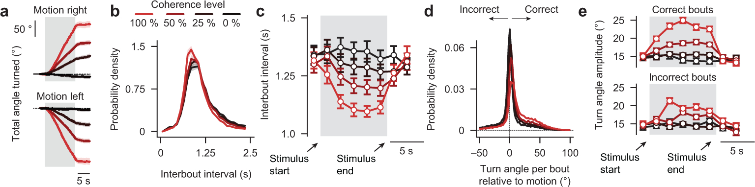
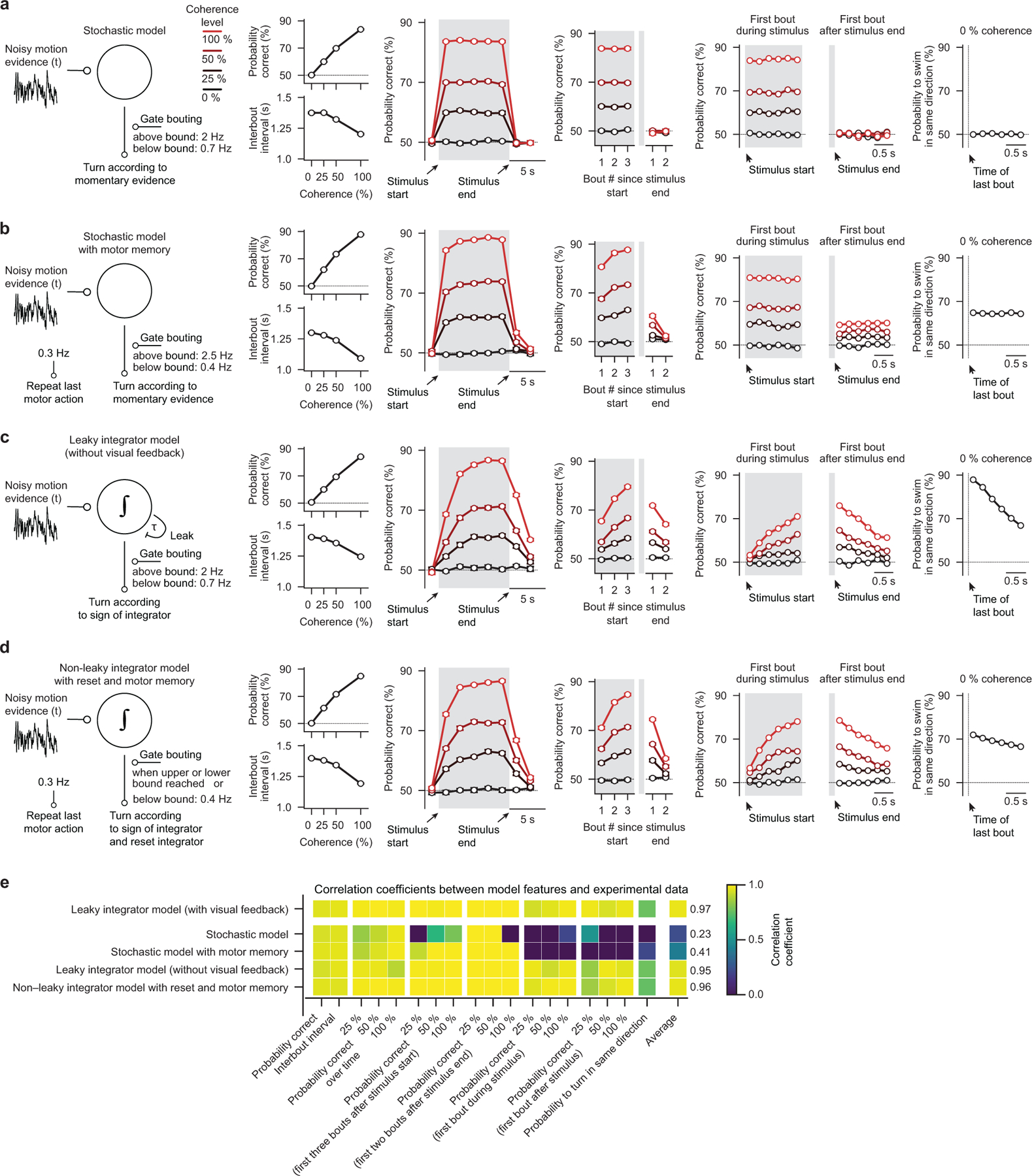
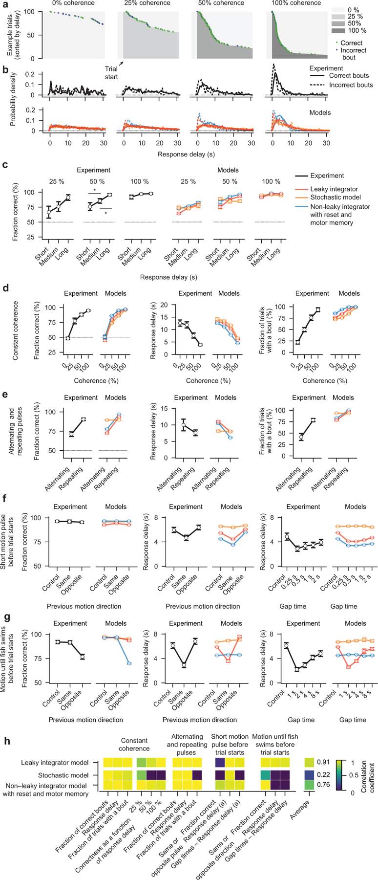
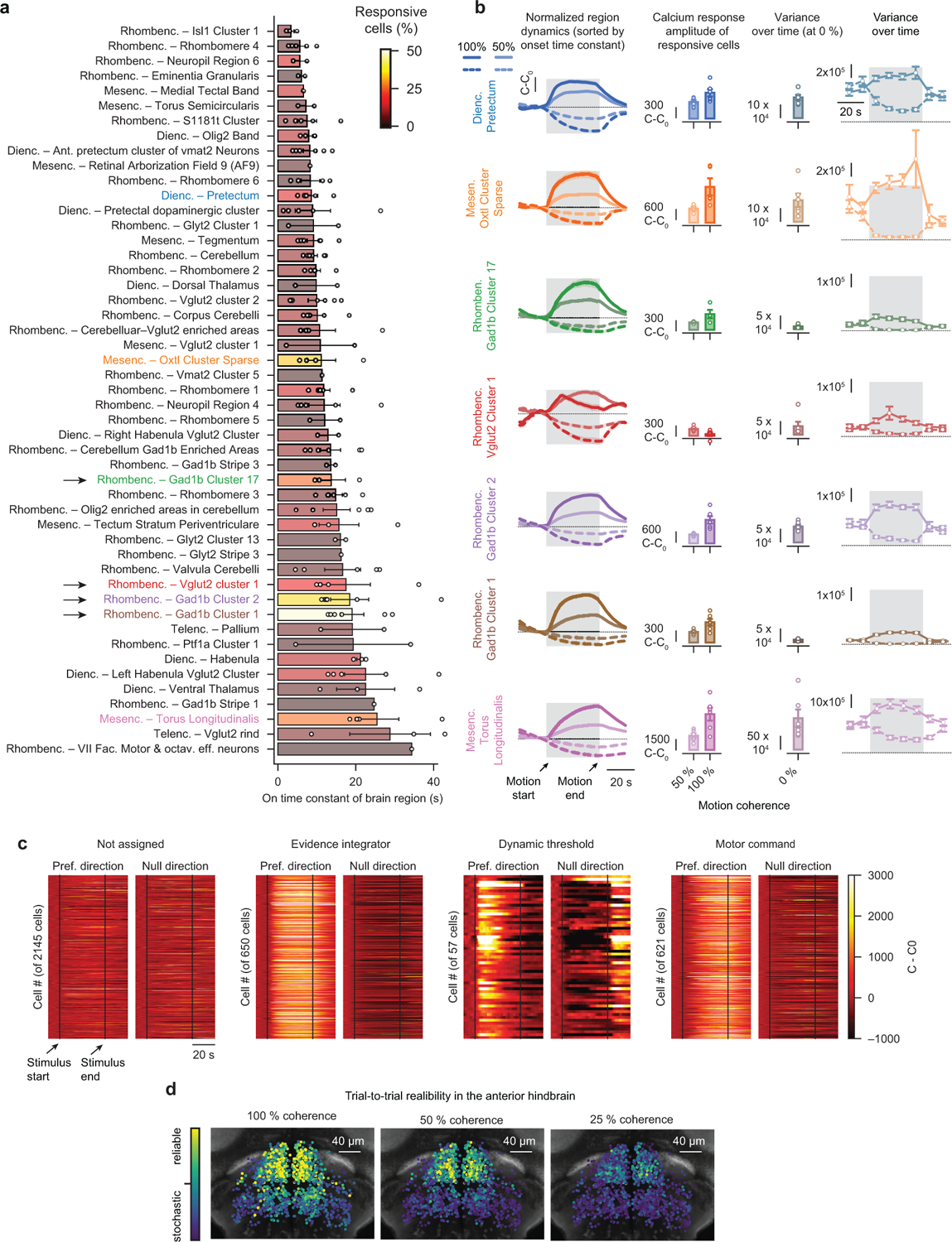
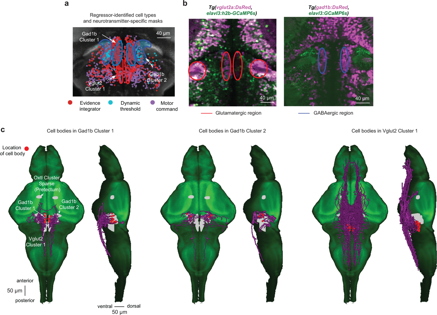
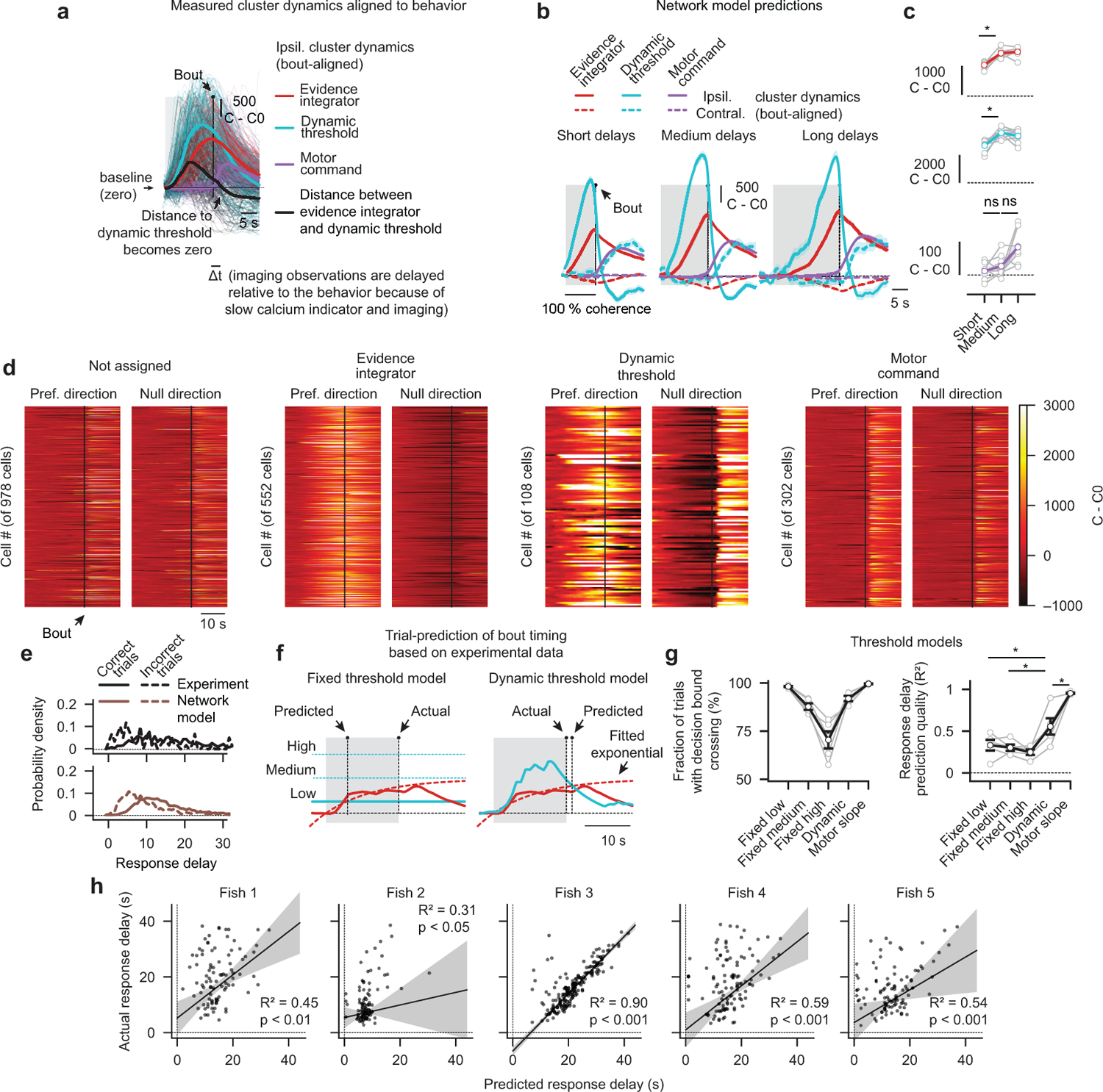
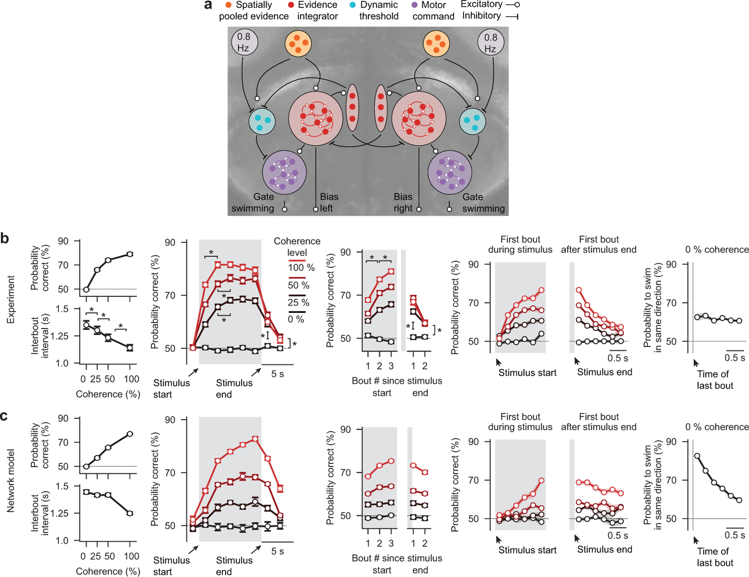
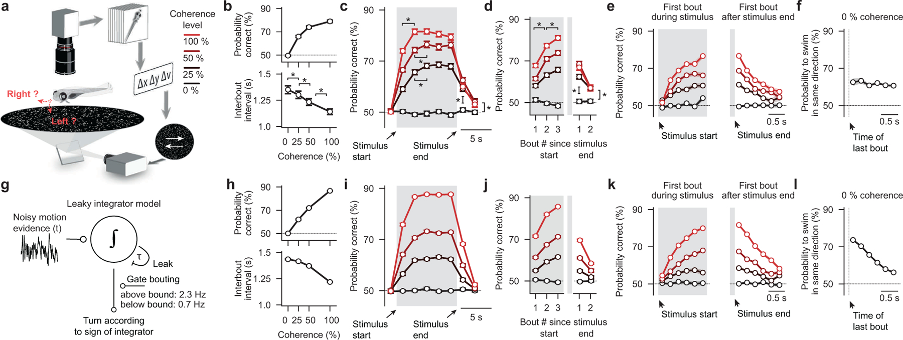
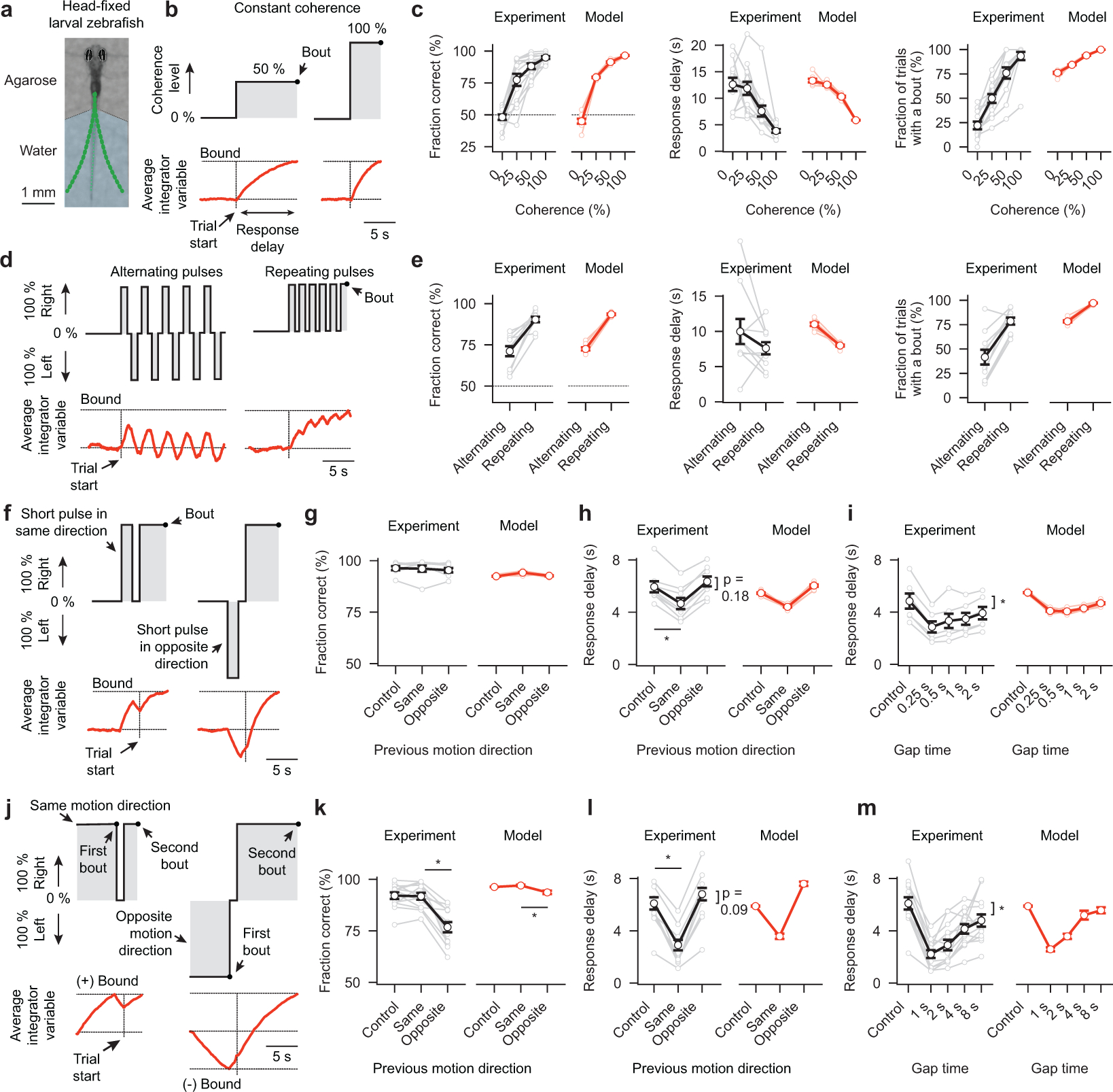
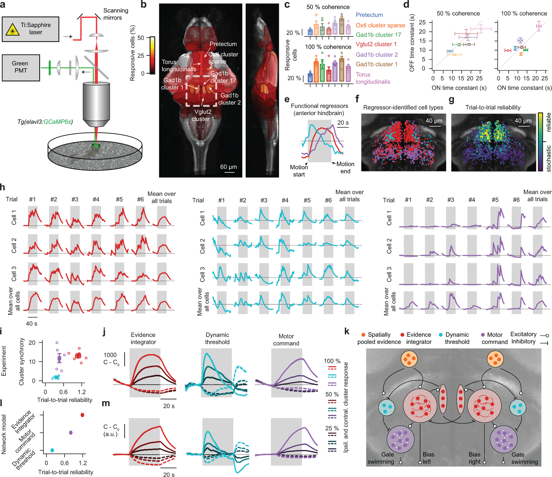
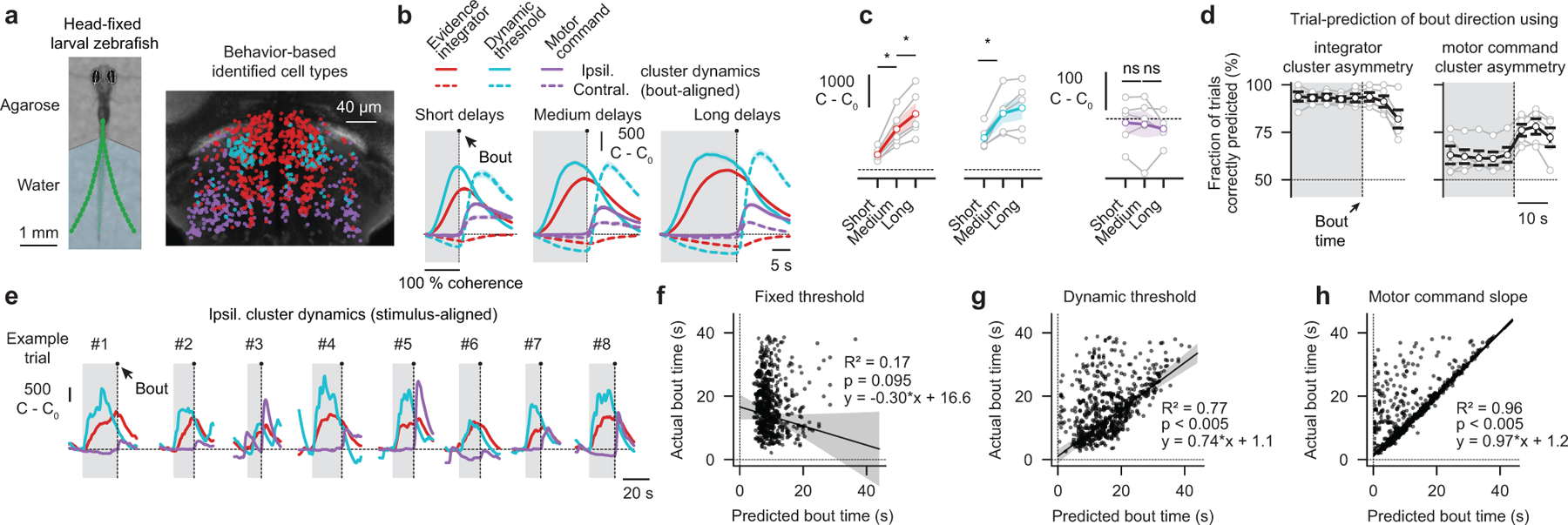
To make appropriate decisions, animals need to accumulate sensory evidence. Simple integrator models can explain many aspects of such behavior, but how the underlying computations are mechanistically implemented in the brain remains poorly understood. Here we approach this problem by adapting the random-dot motion discrimination paradigm, classically used in primate studies, to larval zebrafish. Using their innate optomotor response as a measure of decision making, we find that larval zebrafish accumulate and remember motion evidence over many seconds and that the behavior is in close agreement with a bounded leaky integrator model. Through the use of brain-wide functional imaging, we identify three neuronal clusters in the anterior hindbrain that are well suited to execute the underlying computations. By relating the dynamics within these structures to individual behavioral choices, we propose a biophysically plausible circuit arrangement in which an evidence integrator competes against a dynamic decision threshold to activate a downstream motor command.

Extended Data Fig. 1. Behavior in freely swimming larval zebrafish

a, Turn angle larvae accumulate over time (positive, right; negative, left). b, Probability distribution of interbout intervals during presentation of different coherence levels. c, Time-binned interbout intervals as a function of time. d, Probability distributions of turn angles per bout relative to motion direction. Bouts are defined as correct when they follow motion direction (= positive) and incorrect otherwise (= negative). e, Time-binned precision (absolute turn angle) of correct and incorrect bouts over time. Gray shaded areas in (a,c,e) indicate motion presentation. Before and after, we always show 0 % coherence. Bin sizes in (c,e) are 2 s. All error bars are mean ± sem over fish. N = 60 fish in (a–e), same fish as in Fig. 1b–d.

Extended Data Fig. 2. Model alternatives for freely swimming larval zebrafish

a–d, Schematics and simulation results of alternative models. For simplicity, none of these models had visual feedback. Quantification as in Fig. 1b–f,h–l. N = 16 model runs for each model. e, Pearson’s correlation coefficient between each model feature and the respective experimental data. We use the average of these values to rank the models. All error bars in (a–d) are mean ± sem over model runs.

Extended Data Fig. 3. Behavior and modeling in head-fixed larval zebrafish

a, 100 randomly selected experimental example trials with periods of coherent motion (shades of gray) and 0 % coherence (lightest gray), sorted by response delay. Note that after each correct (green dots) or incorrect (blue dots) bout, coherence levels are immediately set to 0 %. b, Probability density distributions of response delays for correct (solid lines) and incorrect (dashed lines) bouts, for experiment (black lines) and models (red, orange, and blue lines). Models have the same structure as in Extended Data Fig. 2a,c,d but without spontaneous bouts below the bound and different parameters. c, Accuracy as a function of response delay (short: 0–2 s, medium: 2–4 s, long: 4–6 s) for experiment (*p < 0.05 for both comparisons at 50 % coherence) and models. Behavioral data in (a–c) comes from the experiment with constant motion coherence (Fig. 2b). d,e,f,g, Behavior quantification for experiment and models, as in Fig. 2c,e,g–i,k–m. h, Pearson’s correlation coefficient between each model feature and the respective experimental data. We use the average of these values to rank the models. N = 13 fish in (a–d), N = 10 fish in (e), N = 8 fish (left panels) and N = 6 fish (right panel) in (f), N = 13 fish in (g), same fish as in Fig. 2c,e,g–i,k–m. N = 8 model runs for each model in (b–h). All error bars are mean ± sem over fish. P-values in (c) are based on one-sided t-tests comparing response differences to zero. Asterisks (*) in (c) indicate significance (*p < 0.05).

Extended Data Fig. 4. Detailed quantification of responsive brain areas identified during brain-wide calcium imaging

a, All brain areas with >1 % responsive cells, sorted by fitted onset time constant during 50 % coherent motion. Text label colors relate to colors in (b) and Fig. 3c,d. Bar colors represent fraction of responsive cells within a brain region. Black arrows indicate anterior hindbrain regions with slow dynamics and a large fraction of responsive cells. b, Brain areas with >15% responsive cells sorted by temporal dynamics (top, fast; bottom, slow) characterized from left to right. Column 1: Peak-normalized calcium dynamics, relative to baseline (C0) averaged over all cells responding to coherent motion in preferred- (PD) or null-direction (ND), respectively. Column 2: Average (last 5 s of coherent motion) calcium response amplitude (comparisons between 50 % and 100 %, from top to bottom: p = 0.05, p = 0.06, p = 0.16, p < 0.05, p < 0.01, p < 0.05, p < 0.05). Column 3: Variance (over time), calculated in individual cells and trials, then averaged, during 0 % coherence Column 4: Same as column 3 but time-binned for region’s preferred- and null-direction. As variances for preferred- and null-direction motion quickly converge after motion stimulation, the last time bin reflects a motion-memory independent variance at 0 % coherence. c, Preferred- and null-direction dynamics of all identified anterior hindbrain cells functionally clustered by regressor analysis (Fig. 3e). Preferred motion direction refers to motion to the left or right for cells in the left or right hemisphere, respectively, null-direction motion the other way around. d, Spatial arrangement of trial-to-trial reliability for all cells without functional clustering, as in Fig. 3g but for all three coherence levels. N = 6 fish for 50 % and N = 6 fish for 100 % motion coherence stimulation in (a,b). Open circles in (a,b) indicate individual fish. Note that in some fish not all brain areas were imaged and, hence, fish number per brain regions is variable. N = 6 fish in (c,d). All error bars in (a,b) indicate mean ± sem over fish. Shaded gray areas in (b) and dashed vertical lines in (c) indicate motion stimulation. Before and after 0 % coherence is shown. All p-values are based on two-sided t-tests.

Extended Data Fig. 5. Neurotransmitter identity and neuronal morphology in the anterior hindbrain

a, Overlay of neurotransmitter type-specific masks from the z-brain atlas (refs. and 25) (glutamate = red outline; GABA = blue outline) with the functionally characterized cell types (same cells as in Fig. 3f) in the same coordinate system. Note that almost all identified dynamic threshold neurons lie within the Gad1b Cluster 2 and are, therefore, likely inhibitory. Please also note that the expression pattern of the vglut2a-driver line (ref. 25) suggests that the anatomical mask of the VGlut2 Cluster 1 likely extends even further into the anterior part of the hindbrain. b, Simultaneous imaging of DsRed (pink), expressed only in excitatory vglut2a+ neurons (left panel) or of DsRed expressed only in inhibitory gad1b+ neurons (right panel), and cytosolic or nuclear-localized GCaMP6s (green, pan-neuronal expression). Colored ellipses are manually added to highlight regions of interest. c, Single-cell morphologies with somata in the identified regions in the anterior hindbrain. Cells were mapped from the Max-Planck Zebrafish Brain Atlas (ref. 26) into the z-brain coordinate system and overlaid with the available masks (gray) on a GCaMP5G reference larval zebrafish (green). N = 6 fish in (a), same data as in Fig. 3f. N = 1 fish for each plot in (b).

Extended Data Fig. 6. Neural correlates of behavioral choices

a, Measured cluster dynamics aligned to swim bouts (same data as in Fig. 4b but as a reduced version only showing ipsilateral dynamics for medium response delays). The thick black line illustrates the difference between the dynamic threshold cluster and the evidence integrator cluster, which crosses zero (baseline) around the same time the motor command cluster reaches its maximum. This event occurs slightly after the bout likely due to delays introduced by the relatively slow dynamics of the GCaMP6s indicator (ref. 30). The transparent thin lines are single-trial responses. b,c Same analysis as in Fig. 4b,c but for bout-aligned network model simulations (*p < 0.001 for the integrator and dynamic threshold unit comparisons; p = 0.58 and p = 0.06 for the motor command cluster comparisons). d, Bout-aligned preferred- and null-direction dynamics of all identified cells from all N = 5 fish, functionally clustered by the behavior-based classification method. Preferred motion direction refers to motion to the left or right for cells in the left or right hemisphere, respectively, null-direction motion the other way around. e, Probability density distributions of response delays for correct (solid lines) and incorrect (dashed lines) bouts, for experiment (black) and network model (brown). f, Illustration of two methods for trial-by-trial prediction of individual behavioral choices based on the experimentally obtained cluster dynamics. Bouts are predicted when the smoothed and extrapolated integrator cluster activity (red dashed lines are exponential fits of the experimental data, solid red lines) crosses the threshold (cyan lines). Three fixed thresholds (left panel) and the dynamic threshold (right panel) are tested. The third method, which uses a sudden rise in the motor command slope as a predictor, is not illustrated. g, Quantification of the fraction of trials in which a threshold crossing event is detected and quantification of predictive quality (coefficient of determination, R2) for the different threshold models (*p < 0.05 for each model compared to the dynamic threshold model). Gray lines are individual fish, black lines are fish averages. h, Individual fish trial-by-trial predictions of bout-timing using the dynamic threshold, and robust linear regression analysis results (RANSAC, see methods). Gray shaded areas indicate confidence intervals of the regression fits. N = 5 fish in (a,d,e,g,h), same fish as in Fig. 4. N = 8 model runs in (b,c,e). All error bars are mean ± sem over simulated trials in (b), model runs in (c), or fish in (g). P-values in (c,g) are based on one-sided t-tests comparing differences to zero. Asterisks (*) in (c,g) indicate significance (*p < *0.05, or *p < 0.001).

Extended Data Fig. 7. Speculative network model implementation of urgency-related signals in freely swimming larval zebrafish

a, Network model as in Fig. 3k but with inhibitory bout clock attached to the dynamic threshold clusters. We speculate that the bout clock or the system for keeping balance act as urgency-related signals here. These signals lead to rapidly collapsing bounds, allowing for spontaneous swimming. Also, in this model, each simulated bout induced opposing visual feedback, as in Fig. 1g–l. b, Copy of behavior data from Fig. 1b–f. c, Network model simulation results, quantified as in Fig. 1b–f,h–l. N = 8 model runs in (c). All error bars are mean ± sem over fish in (b) or model runs in (c). Asterisks (*) in (b) indicate significance (*p < 0.05, *p < 0.01, or *p < 0.001). See Fig. 1b–f for more details on p-values and statistics.

Figure 1 |. Behavior and modeling in freely swimming larval zebrafish.

a, Random dot motion kinematograms presented from below to freely swimming larval zebrafish. After a few seconds of 0 % coherence (baseline stimulus, no motion, flickering dots), a certain percentage of the dots starts to move coherently either left- or right-ward at a constant speed until we switch coherence levels back to 0 %. Each dot, whether it is moving or not, has a lifetime of a few hundred milliseconds, making it impossible for larvae to track individual dots over the time course of the trial. The system operates in closed-loop so that dots always move perpendicularly to the fish no matter where animals are located and how they are oriented in the arena. Note that sizes are not to scale (the body length a larval zebrafish at this age is ~4 mm, the diameter of the visual arena is 12 cm). b, Accuracy and interbout interval as a function of coherence strength. c, Time-binned accuracy as a function of time (first bin during motion: *p < 0.001 for all coherence levels; second bin during motion: p = 0.9, *p < 0.05, *p < 0.01, for 100 %, 50 %, 25 % coherence level, respectively; first bin after stimulus: *p < 0.001 for all coherence levels; second bin after stimulus: *p < 0.05, *p < 0.01, *p < 0.01, for 100 %, 50 %, 25 % coherence level, respectively). d, Accuracy over consecutive bouts (first to second bout after stimulus start: *p < 0.001, for all coherences; second to third bout after stimulus start: *p < 0.001, *p < 0.01, *p < 0.05, for 100 %, 50 %, 25 % coherence level, respectively; first and second bout relative to 0 % control: *p < 0.001, for all coherences). e, Accuracy of the first bout during the stimulus and the first bout after the stimulus end as a function of delay. f, Probability to swim in the same direction as a function of interbout interval during 0 % coherence. g, Schematic of the bounded leaky integrator model. h–l, Quantification of model simulation results as in (b–f). N = 60 fish in (b–d,f) and N = 56 fish in (e). N = 16 model runs in (h–l). Gray shaded areas in (c–e,i–k) indicate time of motion coherence presentation, before and after coherence levels are at 0 %. All error bars are mean ± sem over fish. P-values are based on one-sided t-tests comparing response differences to zero. All asterisks (*) indicate significance (*p < 0.05, *p < 0.01, or *p < 0.001).

Figure 2 |. Behavior and modeling in head-fixed larval zebrafish.

a, Photograph of a head-fixed larval zebrafish in transparent agarose with the tail free to move. Green dots indicate tail tracking points. In such a preparation, spontaneous swim rates are low, but animals still respond robustly to motion. We track behavioral choices based on the first bout during the trial. b,d,f,j, Stimulation protocols used (black lines with shaded gray area) and cartoons depicting respective estimates of the average bounded leaky integrator variable (red traces). c, Accuracy, response delay, and fraction of trials with a bout as a function of coherence strength. e, Same as in (c) but for stimulation protocol with alternating and repeating motion pulses. g,h, Accuracy and response delay as a function of direction of a single motion pulse shown before the trial. Control conditions have no such pulse (*p < 0.001 for same direction against control). i, Response delay as a function of gap time (0 % coherence) since a same direction motion pulse (*p < 0.001 for gap times 0.25, 0.5, and 1 s; *p < 0.01 for gap time 2 s). k,l,m, Same is in (g,h,i) but with the previous motion stimulus presented until a first bout event (*p < 0.001 for all conditions). Gray and black lines in (c,e,g–i,k–m) indicate individual and average larvae responses, light red and red lines model evaluations, respectively. N = 13 fish in (c), N = 10 fish in (e), N = 8 fish in (g,h), N = 6 fish in (i), N = 13 fish in (k–m), N = 8 model evaluations (different noise seeds) in (c,e,g–i,k–m). All error bars are mean ± sem over fish or model runs. P-values are based on one-sided t-tests comparing response differences to zero. All asterisks (*) indicate significance (*p < 0.05, *p < 0.01, or *p < 0.001).

Figure 3 |. Brain-wide and anterior hindbrain two-photon calcium imaging.

a, Schematic of the two-photon microscope. Fully agarose-embedded animals (no behavior) are presented with dot motion stimuli from below that either drift left- or right-ward. We either image across the entire brain (b–d) or focus on a single plane within the anterior hindbrain (e–j). b, Overlay of all brain regions where the fraction of responsive neurons is larger than 1 % during 50 % coherent motion, on top of z and x projections of the larval zebrafish reference brain. Colors indicate the fraction of responsive cells in the area. Region names follow reference brain (https://engertlab.fas.harvard.edu/Z-Brain) convention. The dashed square indicates where the anterior hindbrain resides. c,d, Quantification of the fraction of responsive cells within the identified brain areas (c) and of regional onset and offset time constant dynamics (d) for 50 % and 100 % coherence levels. e–g, Functional regressors found by k-means clustering (e) and spatial arrangement of clustered cell types (f) together with their trial-to-trial reliability at 50 % coherence (g) for the single plane anterior hindbrain imaging experiment. h, Single cell and trial example dynamics for each identified anterior hindbrain cluster and respective averages over trials and cells for 100 % coherent motion. i, Trial-to-trial reliability plotted against cluster synchrony for each cluster (see methods for metrics). j, Cluster average calcium dynamics, relative to baseline (C₀), for different coherence levels (moving right- or left-ward) over time. Ipsilateral indicates the left or the right hemisphere for left- or right-ward motion, respectively, contralateral the other side. k, Suggested network model. Each cluster is implemented as a single rate unit. l,m, Analysis as in (i,j) but for network model simulations. Cluster synchrony is not defined here as model clusters are single rate units. N = 6 fish for each coherence level in (b–d) and N = 6 fish in (e–j). N = 8 model simulations in (l,m). All error bars indicate mean ± sem over trials (j,m) or fish (c,d,i,l). Gray shaded areas in (e,h,j,m) indicate motion stimulation (before and after, 0 % coherence is shown). Open circles in (c,i) show individual fish.

Figure 4 |. Neural correlates of behavioral choices in the anterior hindbrain.

a, Photograph of a head-fixed larval zebrafish in the two-photon microscope (left panel). Green dots indicate tail tracking points. In each trial, we presented 0 % coherence as a baseline, followed by left- or right-ward moving 100 % coherence until the animal initiated a swim bout. Whenever we detected such an event, we immediately dropped coherence levels to 0 %, which was necessary to prevent vigorous movements and struggles. We used a behavior-based classification approach to determine the functional identity of cell types (right panel). b, Experimentally obtained bout-aligned cluster averages, grouped by response delay (short: 4–10 s, medium: 10–16 s long: 16–22 s). Ipsilateral indicates the left or the right hemisphere for left- or right-ward motion, respectively, contralateral the other side. Gray shaded areas indicate motion stimulation. c, Quantification of ipsilateral cluster activity at bout time as a function of delay (*p < 0.01 for both integrator cluster comparisons; *p < 0.05 for the dynamic threshold cluster comparison; p = 0.72 and p = 0.61 for the motor command cluster comparisons). See Extended Data Fig. 6b,c for model simulations. d, Trial-to-trial prediction of swimming direction, based on the integrator or motor command cluster dynamics, as a function of time relative to bout. e, Example trials of stimulus-aligned ipsilateral cluster dynamics. f,g,h, Trial-to-trial bout time predictions (black dots indicate individual bouts) based on three threshold models and respective robust linear regression analyses (RANSAC, see methods). Gray shaded areas indicate confidence intervals of the regression fits. N = 5 fish in (a–d,f–h) and N = 1 fish in (e). Gray lines with open circles in (c,d) are individual fish, colored or black lines in (c,d) are fish averages. All error bars indicate mean ± sem over trials (b) or fish (c,d). P-values in (c) are based on one-sided t-tests comparing response differences to zero. All asterisks (*) indicate significance (*p < 0.05, *p < 0.01, or *p < 0.001).

References

1. Shadlen MN & Kiani R Decision making as a window on cognition. Neuron 80, 791–806 (2013). - PMC - PubMed
1. Ratcliff R, Smith PL, Brown SD & McKoon G Diffusion decision model: Current issues and history. Trends Cogn. Sci 20, 260–281 (2016). - PMC - PubMed
1. Groschner LN, Chan Wah Hak L, Bogacz R, DasGupta S & Miesenböck G Dendritic integration of sensory evidence in perceptual decision-making. Cell 173, 894–905 (2018). - PMC - PubMed
1. Borst A & Bahde S Visual information processing in the fly’s landing system. J. Comp. Physiol. A 163, 167–173 (1988).
1. DasGupta S, Ferreira CH & Miesenböck G FoxP influences the speed and accuracy of a perceptual decision in Drosophila. Science 344, 901–904 (2014). - PMC - PubMed
Publication types
LinkOut - more resources