Estimating heritability and genetic correlations from large health datasets in the absence of genetic data

Abstract

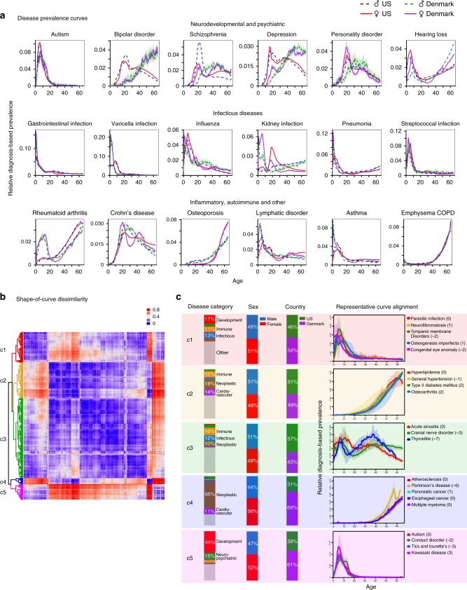
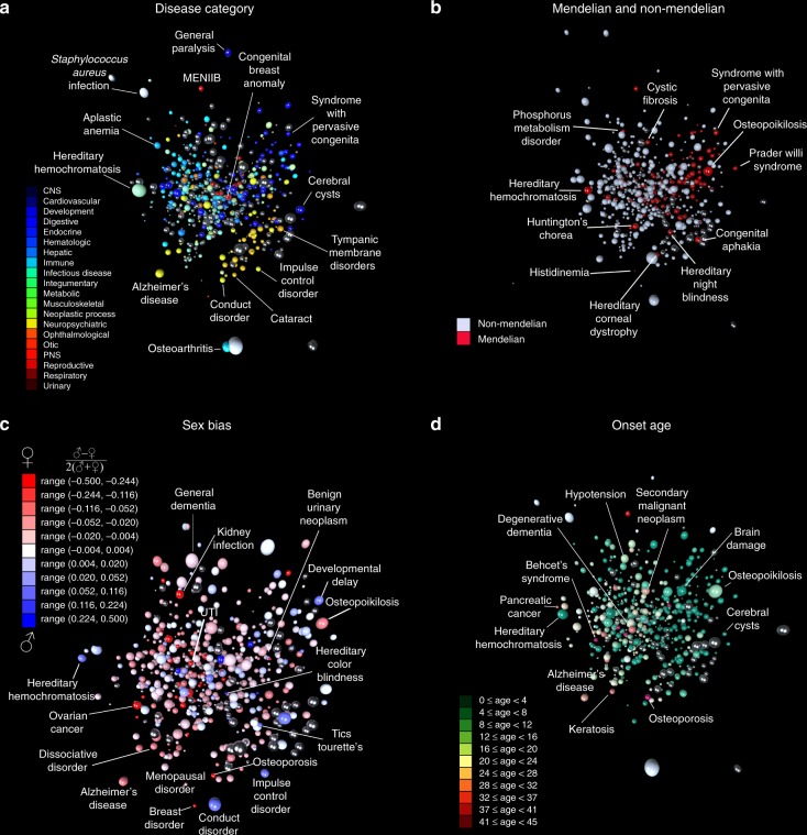
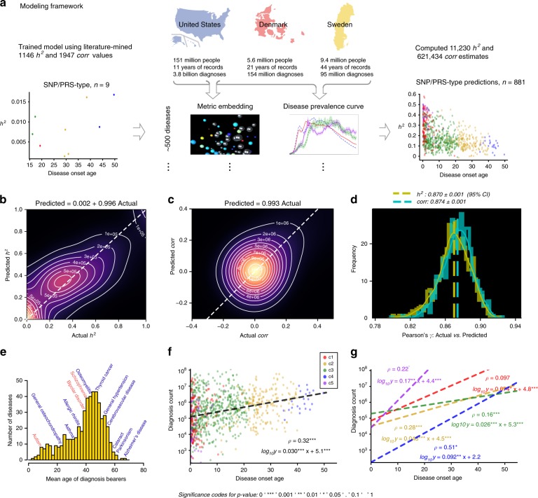
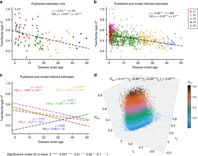
Typically, estimating genetic parameters, such as disease heritability and between-disease genetic correlations, demands large datasets containing all relevant phenotypic measures and detailed knowledge of family relationships or, alternatively, genotypic and phenotypic data for numerous unrelated individuals. Here, we suggest an alternative, efficient estimation approach through the construction of two disease metrics from large health datasets: temporal disease prevalence curves and low-dimensional disease embeddings. We present eleven thousand heritability estimates corresponding to five study types: twins, traditional family studies, health records-based family studies, single nucleotide polymorphisms, and polygenic risk scores. We also compute over six hundred thousand estimates of genetic, environmental and phenotypic correlations. Furthermore, we find that: (1) disease curve shapes cluster into five general patterns; (2) early-onset diseases tend to have lower prevalence than late-onset diseases (Spearman's ρ = 0.32, p < 10^-16); and (3) the disease onset age and heritability are negatively correlated (ρ = -0.46, p < 10^-16).

Fig. 1. Disease prevalence curves fall into five major shape clusters.

a Representative disease prevalence curves for neurodevelopmental, psychiatric, infectious, inflammatory, autoimmune, and some miscellaneous diseases; we show disease names at the top of the corresponding plot. A curve’s x-axis corresponds to the age of diagnoses (not necessarily the first one in the patient’s recorded health trajectory), and the y-axis denotes the relative prevalence of each diagnosis in the corresponding age and sex group. For ease of comparison across countries, we re-normalized each curve to sum to 1. We computed the curves for two countries: the US and Denmark. US male-specific curves are depicted with blue-dotted lines and female-specific ones with red solid lines. As for their Danish counterparts, male-specific curves are shown with green-dotted lines and female-specific ones with purple solid lines. Each curve is supplied with a 99% confidence interval (in transparent colors). We find that some disease curves are consistent across countries and sexes (e.g., autism and gastrointestinal infection), while others vary by country only (e.g., bipolar disorder and rheumatoid arthritis), and still others vary by sex only (e.g., osteoporosis and Crohn’s disease). b A distance matrix, shown as a heatmap, represents the shape dissimilarity between curves measured via the Jensen-Shannon divergence (Methods part 2). We applied a hierarchical clustering algorithm and elbow model selection to arrive at a five-cluster classification of curve shapes; the five clusters, c1–c5, are shown in red, yellow, green, blue, and purple, respectively. c At the left side of the plate, three columns of stacked bar charts summarize the compositions of each cluster in terms of disease category, sex, and country. At the right side of the plate, we show the optimal curve alignments (after relative shifts along the x-axis) of several representative diseases from each cluster. For each disease, we computed variations across four prevalence curve instances (two countries by two sexes), showing the curve mean and variation as a solid line and a shaded same-color area, respectively. The optimal relative shifts for the alignment are written as bracketed integer numbers (in years) after each disease name.

Fig. 2. An embedding disease mapping into metric space positions, with related diseases close to each other.

Diseases can be mapped to points in low-dimensional metric space (so-called “disease embedding”). See the three-dimensional projections of our 20-dimensional embedding in (a)–(d) in this figure, where similar diseases are closer to each other in metric space than dissimilar ones. This 20-dimensional disease embedding turned out to be extremely useful in this study for estimating population-genetics parameters for individual diseases. a We projected the 20-dimensional disease embedding vectors of over 500 diseases into 3-dimensional space for ease of visualization, using the t-SNE algorithm. We color-coded the spheres representing the diseases by each corresponding disease category. Plate b shows Mendelian vs. non-Mendelian disease distribution. Plate c shows disease-specific sex bias (defined in such a way that it is 0 for diseases that are equally frequent in males and females, −0.5 for diseases that occur only in females, and +0.5 for those occurring only in males). Plate d shows diseases color-coded in accordance with their onset ages, where green colors indicate early-onset childhood diseases, and warmer colors point to later-onset diseases.

Fig. 3. Estimating population-genetics parameters for hundreds of diseases and thousands of disease pairs.

Here, h² denotes heritability, and corr is a correlation between a disease pair which can be genetic, environmental, or phenotypic. a A workflow explains the key steps of our model development. We used three national-scale health registries, representing the United States, Denmark, and Sweden, which comprised 3.8 billion, 154 million, and 95 million disease diagnoses, respectively. We computed curves reflecting disease prevalence by age and sex (disease prevalence curves) and derived a metric mapping (disease embedding in metric space) for the whole disease spectrum. We used these two complementary representations to estimate hundreds of thousands of disease-specific parameters. We then validated the accuracy of our model’s predictions by benchmarking them against previously-published (“actual”) estimates that were not used in model training. Plates b and c show kernel density estimation plots we computed from 1000 random 4:1 splits of data (4/5 for training and 1/5 for testing). We used these plots to visualize the joint distribution of the actual data for testing and model-predicted values. The linear fit slopes between the actual and predicted values are 0.996 for h² and 0.993 for corr, indicating nearly perfectly unbiased estimations. d The distributions of Pearson’s correlations between the actual and predicted values have mean values of 0.870 for h² and 0.874 for corr. e A distribution of the mean age of disease-specific diagnosis bearers. The median of the mean ages over all diseases is around 42 years, and specifically, the mean ages of autism, bipolar disorder, and schizophrenia that appeared in the US data are 9, 40, and 41, respectively. f There is a significant positive correlation between disease onset age and diagnosis count in the US data, suggesting there are less-than-expected, rare, late-onset diseases. g The relationship also holds for each of the five disease clusters. For individual clusters (c1–c5), we show the best linear approximation, regression coefficients (p values were computed using Student’s t test), and Spearman’s correlation ρ (p values were computed using algorithm AS 89), color-coded by the shape cluster. Superscript asterisks indicate significance level of the estimates being different from 0.

Fig. 4. Analyses empowered by our estimates of heritability (h²), and genetic and environmental correlations (r_g and r_e).

Plate a includes analyses solely based on the previously published estimates of twin/family-type h², suggesting a significantly negative correlation between disease onset age and heritability. b Our estimator substantially enriched the collection of twin/family-type h² estimates, filling in numerous missing estimates for under-studied diseases. When we analyzed disease prevalence curves jointly, we found a significantly negative correlation between disease onset age and h², which also holds for h² estimates based on other data types, such as SNP/PRS-type (Supplementary Fig. 4b). c We performed the same analysis for diseases within each of the five curve shape clusters, also confirming the significantly negative correlations for shape Clusters 1–3. In the smaller Clusters 4 and 5, the correlations were not significant (Methods part 5). d To understand the relationship between a disease pair’s dissimilarity of disease prevalence curves (D_soc), and the r_g and r_e for the same disease pair, we performed a regression analysis, expressing D_soc as a function of r_g, r_e, and an interaction term r_g·r_e (p values were computed using Student’s t test, see Methods part 6). The corresponding regression coefficients turned out to be 0.41, −0.30, and −0.52, respectively. This regression analysis suggests the following: When two diseases have only high genetic correlation, their prevalence curves are likely to be very different; if only environmental correlation is high, the prevalence curves tend to be much more similar. However, disease prevalence curves are most similar when both environmental and genetic correlations between the two diseases are high. The included disease pairs across all categories are represented as hundreds of thousands of data points in the plot and they are colored according to the D_soc values. We also repeated the same D_soc regression analysis with all disease pairs from distinct disease categories (see Supplementary Data 6 and Supplementary Fig. 5).

References

1. Cover, T. M. & Thomas, J. A. Elements of Information Theory (Wiley-Blackwell, 1991).
1. Ketchen DJ, Shook CL. The application of cluster analysis in strategic management research: an analysis and critique. Strategic Manag. J. 1996;17:441–458. doi: 10.1002/(SICI)1097-0266(199606)17:6<441::AID-SMJ819>3.0.CO;2-G. - DOI
1. Jensen AB, et al. Temporal disease trajectories condensed from population-wide registry data covering 6.2 million patients. Nat. Commun. 2014;5:4022. doi: 10.1038/ncomms5022. - DOI - PMC - PubMed
1. Edwards JH. Familial predisposition in man. Br. Med. Bull. 1969;25:58–64. doi: 10.1093/oxfordjournals.bmb.a070672. - DOI - PubMed
1. Boomsma D, Busjahn A, Peltonen L. Classical twin studies and beyond. Nat. Rev. Genet. 2002;3:872–882. doi: 10.1038/nrg932. - DOI - PubMed
Publication types