Computational modeling demonstrates that glioblastoma cells can survive spatial environmental challenges through exploratory adaptation

Abstract

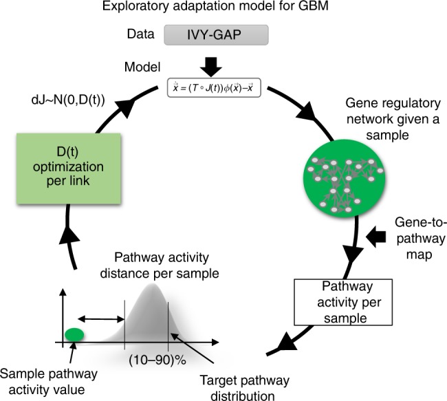
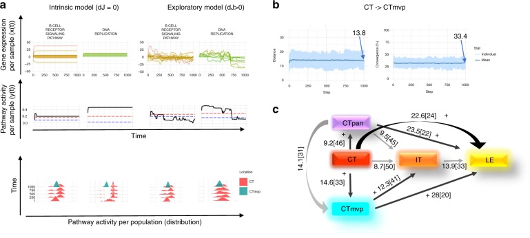
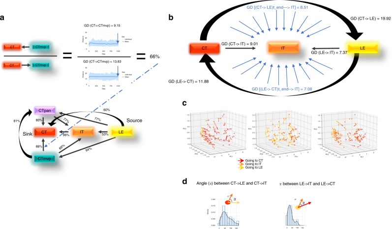
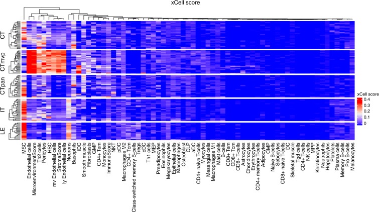
Glioblastoma (GBM) is an aggressive type of brain cancer with remarkable cell migration and adaptation capabilities. Exploratory adaptation-utilization of random changes in gene regulation for adaptive benefits-was recently proposed as the process enabling organisms to survive unforeseen conditions. We investigate whether exploratory adaption explains how GBM cells from different anatomic regions of the tumor cope with micro-environmental pressures. We introduce new notions of phenotype and phenotype distance, and determine probable spatial-phenotypic trajectories based on patient data. While some cell phenotypes are inherently plastic, others are intrinsically rigid with respect to phenotypic transitions. We demonstrate that stochastic exploration of the regulatory network structure confers benefits through enhanced adaptive capacity in new environments. Interestingly, even with exploratory capacity, phenotypic paths are constrained to pass through specific, spatial-phenotypic ranges. This work has important implications for understanding how such adaptation contributes to the recurrence dynamics of GBM and other solid tumors.

Fig. 1. GBM spatial phenotypic trajectories.

Initial analysis of the static data was conducted to assess spatial phenotypic trajectories. Pathways and global distances were calculated for every pair of locations based on population distributions. a Illustration of sampled locations from Ivy GAP datasets, including gene expression data from 41 patients taken from the following anatomic regions: cellular tumor (CT), leading edge (LE), infiltrating tumor (IT), pseudopalisading region around necrosis (CTpan), and microvascular proliferation (CTmvp). Arrows demonstrate the potential spatial tumor spread patterns that we focused on throughout this study. b For each sample, a molecular network was constructed based on our GBM focused gene list, relevant TFs, gene expression, and pathway activities. c A sample’s phenotype is defined to be its vector of pathway activities. For each location, a pathway activity distribution was created based on the pathway activities of all samples from that location. The location’s phenotype was thus defined as a vector of pathway activities distributions. d–g Differences between phenotypes were estimated in several ways: d clustering groups of samples based on their pathway activity patterns (see Supplementary Fig. 1 for more details), e data reduction of pathway activities using BGA. The plot visualizes the spatial trajectories using patterns of pathway activities of all samples, f pathway distributions distances were calculated between every pair of locations. g integrating all those pathway distributions distances between every pair of locations gives a reduced value of global distances, plotted as histogram. h, i Resulting phenotype distances and phenotype spatial trajectories. This complex information can be depicted as a network, where nodes are location’s phenotypes, and edges are distances between phenotypes. The edges’ weights can be estimated in three ways: first (section H), mean of the pathways distribution distances (PD), given as the first value. Second (section I), number of differential pathway activities (DA), given as the second value in brackets, and third, global distances, given in Supplementary Data 1. Based on these three values, shortest paths are as follow: (CT, CTpan), (CT,IT), (CT,CTmvp), (CTpan,IT), and (IT, LE), are marked with dashed lines. All other larger distances are marked with solid lines. PD and DA are strongly correlated across all locations (see Supplementary Data 1 and Supplementary Fig. 1 for a complete list of p-values and correlation coefficients).

Fig. 2. Flow chart of single-sample dynamics model.

At every time step t, the model performs the following steps: (1) the vector of gene expression (x(t)) is updated based using the gene regulatory network, with edges weighted by correlations between the expression of the nodes genes; (2) the phenotype (y(t)) is calculated as the pathway activity vector based on the gene expressions x(t); (3) the minimum distance between the current sample’s phenotype and the 10–90th percentile interval of target’s phenotype distribution is estimated for each pathway; (4) If the distance is 0, that is, the sample’s phenotype is within the target’s phenotype distribution, the exploratory capacity, D(t), decreases relative to its previous time value. This process is repeated until the phenotype converges to its target, or the simulation is stopped at t = 1000.

Fig. 3. Cellular response to known and new environmental stimuli.

a An example depicting the phenotype transition CT→CTmvp: first, for a given sample changes for two example pathways (DNA replication and B cell receptor signaling pathways) and their corresponding genes were plotted over time. The lower panel show the activity distributions of the two example pathways obtained from the set of samples from each location. Simulation showed that the exploratory behaviors of both pathways differ from the intrinsic behaviors, therefore indicating that new adaptive pathway activities are due to the exploratory ability. b Following the calculations in sub-plot A, global distance per sample, together with the number of converged pathways were calculated over time. Light blue color represents individual samples’ temporal phenotype distances, and the dark blue line represents the mean value of that global distance. Initial D (t = 0) was set to 0.1, and the distance (t = 1000) reached 13.83, while number of converged pathways was reached to 33.4% on that time step. c Simulation results of the updated location-based phenotypes were re-calculated to include exploratory capacity (dJ > 0). Black color with a plus sign denote weights that are different from those of the intrinsic behaviors (dJ = 0) (intrinsic behavior is marked with gray lines).

Fig. 4. Properties of the simulated phenotype dynamics.

a The reverse process of transitioning between phenotypes was simulated for each edge of the location-based phenotype network from Fig. 3 (as seen by the reversal of the directions of the edges of the network in Fig. 4 compared to those of the network in Fig. 3). The ratio of global distance differences, and the ratio of number of converged pathways in square brackets, between the two directions are shown as weights. b–d The importance of spatially intermediate phenotype states. Focusing on the trajectory of CT→IT→LE, and the reverse trajectory, we examined three characteristics of the resulting intermediate phenotypes and the reversal process: b the ratios of the global distances between the two paths show that cells reverting their trajectory need smaller changes in phenotype to get back from LE to CT, compared to reaching LE from CT using the original path: they are closer to the target phenotype when reverting (11.88 distance) compared to the original end point (19.92); c vector fields of the simulated phenotype dynamics were plotted using PCA; the arrow origins are the starting phenotypes (t = 0) and the end points are the simulated phenotypes (t = 1000). The color of the dots corresponds to the starting phenotype location, whereas the colors of the arrows depict the target phenotype; for example, red arrows that start from a yellow dot are simulation results of a case where the initial condition is LE, and the target phenotype is CT; D) the angles between the original paths of CT→ LE and CT→IT, and angles between the reversal paths LE→CT and LE→IT are narrow, which indicates a constrained sphenotype exploration space.

Fig. 5. Immune signatures of the phenotypes.

xCell was used to deconvolute the (whole genome) bulk expression profiles of the different Ivy-GAP locations, and obtain the plotted signatures.

References

1. Gilbert MR, et al. A randomized trial of bevacizumab for newly diagnosed glioblastoma. N. Engl. J. Med. 2014;370:699–708. doi: 10.1056/NEJMoa1308573. - DOI - PMC - PubMed
1. Chinot OL, et al. Bevacizumab plus radiotherapy-temozolomide for newly diagnosed glioblastoma. N. Engl. J. Med. 2014;370:709–722. doi: 10.1056/NEJMoa1308345. - DOI - PubMed
1. Chamberlain MC. Radiographic patterns of relapse in glioblastoma. J. Neurooncol. 2011;101:319–323. doi: 10.1007/s11060-010-0251-4. - DOI - PubMed
1. Schreier HI, Soen Y, Brenner N. Exploratory adaptation in large random networks. Nat. Commun. 2017;8:14826. doi: 10.1038/ncomms14826. - DOI - PMC - PubMed
1. Braun E. The unforeseen challenge: from genotype-to-phenotype in cell populations. Rep. Prog. Phys. 2015;78:036602. doi: 10.1088/0034-4885/78/3/036602. - DOI - PubMed
Publication types