Delay in recovery of the Antarctic ozone hole from unexpected CFC-11 emissions

Abstract

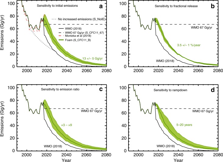
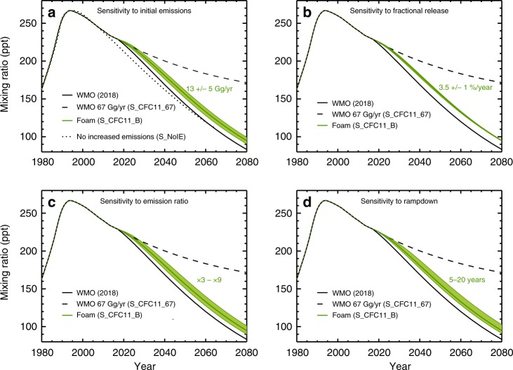
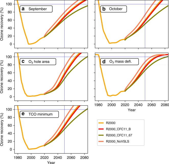
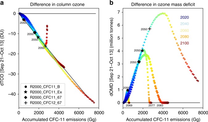
The Antarctic ozone hole is decreasing in size but this recovery will be affected by atmospheric variability and any unexpected changes in chlorinated source gas emissions. Here, using model simulations, we show that the ozone hole will largely cease to occur by 2065 given compliance with the Montreal Protocol. If the unusual meteorology of 2002 is repeated, an ozone-hole-free-year could occur as soon as the early 2020s by some metrics. The recently discovered increase in CFC-11 emissions of ~ 13 Gg yr^-1 may delay recovery. So far the impact on ozone is small, but if these emissions indicate production for foam use much more CFC-11 may be leaked in the future. Assuming such production over 10 years, disappearance of the ozone hole will be delayed by a few years, although there are significant uncertainties. Continued, substantial future CFC-11 emissions of 67 Gg yr^-1 would delay Antarctic ozone recovery by well over a decade.

Fig. 1. Past and potential future emissions of CFC-11.

Estimated emissions of CFC-11 for the past derived from atmospheric measurements and for future scenarios with different assumptions. a Five scenarios including the World Meteorological Organisation (WMO) (2018) baseline scenario (solid black line) and an assumption of constant 67 Gg yr⁻¹ emissions (dashed line, S_CFC11_67). Also shown is a scenario with decreasing emissions from an estimate of the 2002 bank (dotted line, S_NoIE). Emissions based on box model simulations for unreported CFC-11 production for foam use are shown in green (solid line, S_CFC11_B). The green shading indicates the sensitivity range for S_CFC11_B for initial emissions ranging from 8 to 18 Gg/yr (see Methods for assumptions). b Similar to panel a, for WMO (2018) baseline and S_CFC11_67 scenarios with green shading showing sensitivity of scenario S_CFC11_B for fractional release ranging from 2.5 to 4.5%/year. c Similar to panel b, and showing sensitivity to emission ratios from ×3 to ×9. d Similar to panel b, and showing sensitivity to rampdown of new production between 5 and 20 years.

Fig. 2. Past and potential future concentrations of CFC-11.

As Fig. 1 but for CFC-11 volume-mixing ratio (ppt). a Four scenarios including the World Meteorological Organisation (WMO) (2018) baseline scenario (solid black line) and an assumption of constant 67 Gg yr⁻¹ emissions (dashed line, S_CFC11_67). Also shown is a scenario with decreasing emissions from an estimate of the 2002 bank (dotted line, S_NoIE). Emissions based on box model simulations for unreported CFC-11 production for foam use are shown in green (solid line, S_CFC11_B). The green shading indicates the sensitivity range for S_CFC11_B for initial emissions ranging from 8 to 18 Gg/yr (see Methods for assumptions). b Similar to panel a, for WMO (2018) baseline and S_CFC11_67 scenarios with green shading showing sensitivity of scenario S_CFC11_B for fractional release ranging from 2.5 to 4.5%/year. c Similar to panel b, and showing sensitivity to emission ratios from ×3 to ×9. d Similar to panel b, and showing sensitivity to rampdown of new production between 5 and 20 years.

Fig. 3. Antarctic ozone and metrics quantifying ozone loss as a function of meteorology and additional CFC-11 emissions.

Mean column ozone (DU) averaged from 90^oS to 60^oS for a September and b October from TOMCAT simulations CNTL (control), fODS (fixed ozone-depleting substances), R2000, R2002, R2009, R2010 (repeating meteorology from 2000, 2002/2003, 2009/2010 and 2010/2011, respectively), R2000_NoIE (no increased CFC-11 emissions), R2000_NoVSLS (no chlorinated very short-lived substances), R2000_CFC11_67 (with constant CFC-11 emissions of 67 Gg yr⁻¹), R2000_CFC11_B and R2010_CFC11_B (with additional CFC-11 emissions from box model for 2000 and 2010/2011 meteorology, respectively) (see legend) from 1960 to 2090. Panel b also shows mean (±1σ cyan shading) chemistry-climate modelling initiative (CCMI) results. Estimates of the size of the Antarctic ozone hole using c area contained within the 220 DU contour (×10⁶ km²) (averaged September 7–October 13), d ozone mass deficit (×10⁶ tonnes) (averaged September 21–October 13) and e minimum column ozone (between September 21 and October 16). All panels also show observations (black line) from NASA Solar Backscatter Ultraviolet (SBUV) instrument (a, b) or https://ozonewatch.gsfc.nasa.gov/statistics/annual_data.htm (c–e). The coloured dots on the fODS line (panels a, b) show the years used for simulations R2000, R2002, R2009 and R2010. The pink line in the background in all panels from 2018 to 2090 shows the results of the continuation of run CNTL with 20-year repeating meteorology.

Fig. 4. Past and simulated future Arctic ozone showing the influence of meteorology and additional CFC-11 emissions.

Mean column ozone (DU) averaged from 90^oN to 60^oN for a February and b March from TOMCAT simulations CNTL (control), fODS (fixed ozone-depleting substances), R2000, R2002, R2009, R2010 (repeating meteorology from 2000, 2002/2003, 2009/2010, and 2010/2011, respectively), R2000_NoIE (no increased CFC-11 emissions), R2000_NoVSLS (no chlorinated very short-lived substances), R2000_CFC11_67 (with constant CFC-11 emissions of 67 Gg yr⁻¹), R2000_CFC11_B and R2010_CFC11_B (with additional CFC-11 emissions from box model for 2000 and 2010/2011 meteorology, respectively) (see legend) from 1960 to 2090. Panel b also shows mean (±1σ shading) chemistry-climate modelling initiative (CCMI) results from Dhomse et al. and observations from NASA Solar Backscatter Ultraviolet (SBUV) instrument (black line). The coloured dots on the fODS line show the years used for simulations R2000, R2002, R2009 and R2010. The pink line in the background from 2018 to 2090 shows results of the continuation of run CNTL with 20-year repeating meteorology.

Fig. 5. Extent of recovery for Antarctic ozone hole showing the influence of varying chlorine loading.

Extent of recovery (%) for the metrics of a September mean column ozone (90^oS–60^oS), b October mean column ozone, c area contained within the 220 DU contour (averaged September 7–October 13), d ozone mass deficit (averaged September 21–October 13) and e minimum column ozone (between September 21 and October 16) from TOMCAT simulations R2000 (2000 meteorology), R2000_CFC11_B (with additional CFC-11 emissions from box model), R2000_CFC11_67 (with constant CFC-11 emissions of 67 Gg yr⁻¹) and R2000_NoVSLS (no chlorinated very short-lived substances) (see legend) from 1980 to 2080. For the metrics 0% recovery is defined as the maximum depletion (which occurs around 1998) and 100% recovery is defined as return to the 1980 value. The blue horizontal and vertical lines indicate 100% recovery and 2050, respectively.

Fig. 6. Antarctic ozone depletion versus accumulated chlorine emissions.

a The mean column ozone difference (DU) between run R2000 (2000 meteorology) and runs R2000_CFC11_B (with additional CFC-11 emissions from box model, circle), R2000_CFC11_67 (with constant CFC-11 emissions of 67 Gg yr⁻¹, diamond) and R2000_CFC12_67 (with constant CFC-11 emissions of 67 Gg yr⁻¹ and CFC-12 emissions of 59 Gg yr⁻¹, + symbol) in regions 60^oS–90^oS for the period September 21–October 13 (corresponding to the time period for the ozone mass deficit metric in Fig. 3) is plotted against accumulated additional equivalent CFC-11 emissions (Gg). Also shown are the results for simulation R2000_CFC11_Ex (star, see Supplementary Information). The colour shading indicates the year for each data point; the points for 2050 are plotted in black. The slope of best-fit line through the 2050 data points is 0.6 DU/100 Gg CFC-11. b Difference in estimated ozone mass deficit (million tons) versus accumulated equivalent CFC-11 emissions for the same simulations as panel (a).

References

1. Molina MJ, Rowland FS. Stratospheric sink for chlorofluoromethanes: chlorine atom-catalysed destruction of ozone. Nature. 1974;249:810–812. doi: 10.1038/249810a0. - DOI
1. Farman JC, Gardiner BG, Shanklin JD. Large losses of total ozone in Antarctica reveal seasonal ClOx/NOx interaction. Nature. 1985;315:207–210. doi: 10.1038/315207a0. - DOI
1. Engel, A., et al. Update on ozone-depleting substances (ODSs) and other gases of interest to the Montreal Protocol. Chapter 1 in Scientific Assessment of Ozone Depletion 2018 (World Meteorological Organization, Geneva, Switzerland, 2018).
1. World Meteorological Organisation (WMO). Scientific Assessment of Ozone Depletion: 2018, Global Ozone Research and Monitoring Project—Report No. 58. (2018).
1. Froidevaux L, et al. Temporal decrease in upper atmospheric chlorine. Geophys. Res. Lett. 2006;33:8–12. doi: 10.1029/2006GL027600. - DOI
Publication types