From QTLs to Adaptation Landscapes: Using Genotype-To-Phenotype Models to Characterize G×E Over Time

Abstract

Genotype by environment interaction (G×E) for the target trait, e.g. yield, is an emerging property of agricultural systems and results from the interplay between a hierarchy of secondary traits involving the capture and allocation of environmental resources during the growing season. This hierarchy of secondary traits ranges from basic traits that correspond to response mechanisms/sensitivities, to intermediate traits that integrate a larger number of processes over time and therefore show a larger amount of G×E. Traits underlying yield differ in their contribution to adaptation across environmental conditions and have different levels of G×E. Here, we provide a framework to study the performance of genotype to phenotype (G2P) modeling approaches. We generate and analyze response surfaces, or adaptation landscapes, for yield and yield related traits, emphasizing the organization of the traits in a hierarchy and their development and interactions over time. We use the crop growth model APSIM-wheat with genotype-dependent parameters as a tool to simulate non-linear trait responses over time with complex trait dependencies and apply it to wheat crops in Australia. For biological realism, APSIM parameters were given a genetic basis of 300 QTLs sampled from a gamma distribution whose shape and rate parameters were estimated from real wheat data. In the simulations, the hierarchical organization of the traits and their interactions over time cause G×E for yield even when underlying traits do not show G×E. Insight into how G×E arises during growth and development helps to improve the accuracy of phenotype predictions within and across environments and to optimize trial networks. We produced a tangible simulated adaptation landscape for yield that we first investigated for its biological credibility by statistical models for G×E that incorporate genotypic and environmental covariables. Subsequently, the simulated trait data were used to evaluate statistical genotype-to-phenotype models for multiple traits and environments and to characterize relationships between traits over time and across environments, as a way to identify traits that could be useful to select for specific adaptation. Designed appropriately, these types of simulated landscapes might also serve as a basis to train other, more deep learning methodologies in order to transfer such network models to real-world situations.

Keywords: APSIM model; G×E interaction; QTL (quantitative trait loci); adaptation; crop growth model; reaction norm; wheat.

Figure 1

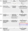
Steps to generate the adaptation landscape. Bottom left; an Australian wheat panel is defined as a sample of the target population of genotypes (TPG). For this set of wheat lines, the genotypes were characterized by SNP markers, phenotypic data have been collected in field trials. The phenotypic and genetic data were used in univariate GWAS analyses to estimate empirical distributions for the additive effects of QTLs underlying these phenotypes. Physiological knowledge on trait correlations was used to define genetic correlations between APSIM parameters $(y_i^P)$. These correlations are included in a multi-variate description of the QTLs underlying APSIM parameters. From this distribution, genotype specific APSIM parameters $(y_i^P)$ are generated and assigned to a subset of SNPs. Bottom right; 31 years of historical environmental data at four sites were used to define the target population of environments (TPE) and identify contrasting environment scenarios (water deficit patterns). Top panel; the environmental data of the selected scenarios and the genotype-dependent APSIM parameters are used to generate intermediate traits over time $(y_{ij}^I)$ using APSIM. The target trait $(y_{ij}^T)$ is modeled as a function of intermediate traits.

Figure 2

Steps to generate the genotype-dependent parameters, additive effects sampled with copulas from a marginal distribution that follows the same shape and rate than the ones of real wheat data. Steps were as follows: (1) define the distribution of the underlying additive effects by fitting empirical distributions of additive effects estimated from a genome-wide association scan (GWAS) applied to wheat heading date and yield in Australia, (2) sample the additive effects from gamma marginal distributions using copulas, (3) attach the sampled additive effects to 300 SNPs randomly sampled and in low linkage disequilibrium with each other. Alleles for heading date were attached to known flowering time genes. The fixation index (Fst) was calculated for each of the 300 SNPs to assess its potential confounding with population structure. (4) For each APSIM parameter, define which will be the trait-increasing allele, so that target parameter correlations are met, and (5) rescale parameters to meet the range that is biologically relevant for this target population of genotypes (TPG).

Figure 3

Population structure as revealed by principal components extracted from the matrix of marker scores. Color symbols indicate the genotype assignment to one of the five sub-populations. Directions of greatest change for a set of physiological parameters have been projected on the biplots to help in interpretation. The length of the physiological parameter representations is proportional to the amount of variation explained by the kinship principal components.

Figure 4

APSIM simulated water supply–demand ratio (stress index) for a genotype with average parameter values growing in Emerald, Narrabri, Merredin, and Yanco during 1983–2013, considering windows of 100^oCd. Thermal time was expressed as cumulative degree days from flowering as computed by APSIM. The water supply/demand ratio indicates the degree to which the soil water extractable by the roots (water supply) is able to match the potential transpiration (water demand). The water demand (mm) corresponds to the amount of water the crop would have transpired in the absence of soil water constraint and is estimated on a daily basis from the amount of crop growth on that day (g mm^–2), and the atmospheric saturation vapor pressure deficit (kPa, Chapman et al., 2000b; Chenu et al., 2011). Line colors correspond to the four environment types obtained by hierarchical clustering of all location × year combinations together. Pie charts represent the frequency of occurrence of environment types at each location for the 31 year period.

Figure 5

AMMI biplot for simulated grain yield (kg ha⁻¹) in Emerald, Merredin, Narrabri, and Yanco during 1983–2013. Circles represent genotype scores (colored by groups) and arrows represent environment scores (colored by environment type).

Figure 6

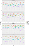
Prediction accuracy and standard error for environments in Emerald, Merredin, Narrabri, and Yanco, between 1983–2013. 20 training sets with four environments randomly drawn from each of the four environment types were used to train the following models: ETmean (yield predicted per environment type, using an unstructured model for environment types), FReg (factorial regression model), IndivPC (independent model terms for each of the cross-products between four genotypic and three environmental scores), MeanPC (mean of the cross-products of genotypic and environment scores).

Figure 7

Upper panels: For three location/year combinations, the correlation between daily phenotypes for secondary traits and grain yield at the end of the growing season, and correlation between APSIM parameters (which are a single constant for each genotype) and daily biomass (dark blue indicates a correlation of +1 and dark red indicates a correlation of −1). The correlation between APSIM parameters and grain yield at the end of the growing season is shown between the blue vertical bars. Vertical lines indicate mean phenology for the population, expressed as Zadoks scores for the population mean (Z2.1 is the beginning of tillering, Z3.1 is the beginning of stem elongation, Z5.5 is heading and Z6.5 is anthesis). Lower panels: water supply/demand ratio for the population mean, calculated for sliding windows of 100 ^oCd from sowing.

Figure 8

Upper panels: For three location/year combinations, the daily biomass production (kg ha⁻¹) for the 199 wheat genotypes. Lower panels: QTL additive effects for biomass estimated from the GWAS for the daily APSIM output. QTL additive effects are expressed as a percentage of the population mean at a given environment and day. SNPs are grouped based on their effects on the APSIM parameters. APSIM parameters written in blue are increased by the most frequent SNP allele, whereas APSIM parameters written in red are decreased by the most frequent SNP allele. Vertical lines indicate mean phenology for the population, expressed as Zadoks scores for the population mean (Z2.1 is the beginning of tillering, Z3.1 is the beginning of stem elongation, Z5.5 is heading and Z6.5 is anthesis). The effect (kg ha⁻¹) of the biomass QTLs on final grain yield at the end of the growing season is shown between the blue vertical bars.

References

1. Álvaro F., Isidro J., Villegas D., García del Moral L. F., Royo C. (2008). Breeding effects on grain filling, biomass partitioning, and remobilization in Mediterranean durum wheat. Agron. J. 100, 361–370. 10.2134/agrojnl2007.0075 - DOI
1. Acreche M. M., Briceño-Félix G., Martín Sánchez J. A., Slafer G. A. (2009). Radiation interception and use efficiency as affected by breeding in Mediterranean wheat. F. Crop Res. 110, 91–97. 10.1016/j.fcr.2008.07.005 - DOI
1. Asseng S., Keating B. A., Fillery I. R. P., Gregory P. J., Bowden J. W., Turner N. C., et al. (1998). Performance of the APSIM-wheat model in Western Australia. F. Crop Res. 57, 163–179. 10.1016/S0378-4290(97)00117-2 - DOI
1. Atlin G. N., Kleinknecht K., Singh G. P., Piepho H. P. (2011). Managing genotype x environment interaction in plant breeding programs: a selection theory approach. J. Indian Soc Agric. Stat. 65, 237–247.
1. Bogard M., Ravel C., Paux E., Bordes J., Balfourier F., Chapman S. C., et al. (2014). Predictions of heading date in bread wheat (Triticum aestivum L.) using QTL-based parameters of an ecophysiological model. J. Exp. Bot. 65, 5849–5865. 10.1093/jxb/eru328 - DOI - PMC - PubMed
LinkOut - more resources