Genomic evidence supports a clonal diaspora model for metastases of esophageal adenocarcinoma

Abstract

The poor outcomes in esophageal adenocarcinoma (EAC) prompted us to interrogate the pattern and timing of metastatic spread. Whole-genome sequencing and phylogenetic analysis of 388 samples across 18 individuals with EAC showed, in 90% of patients, that multiple subclones from the primary tumor spread very rapidly from the primary site to form multiple metastases, including lymph nodes and distant tissues-a mode of dissemination that we term 'clonal diaspora'. Metastatic subclones at autopsy were present in tissue and blood samples from earlier time points. These findings have implications for our understanding and clinical evaluation of EAC.

Extended Data Fig. 1. Flowchart describing key steps taken to construct phylogenetic trees

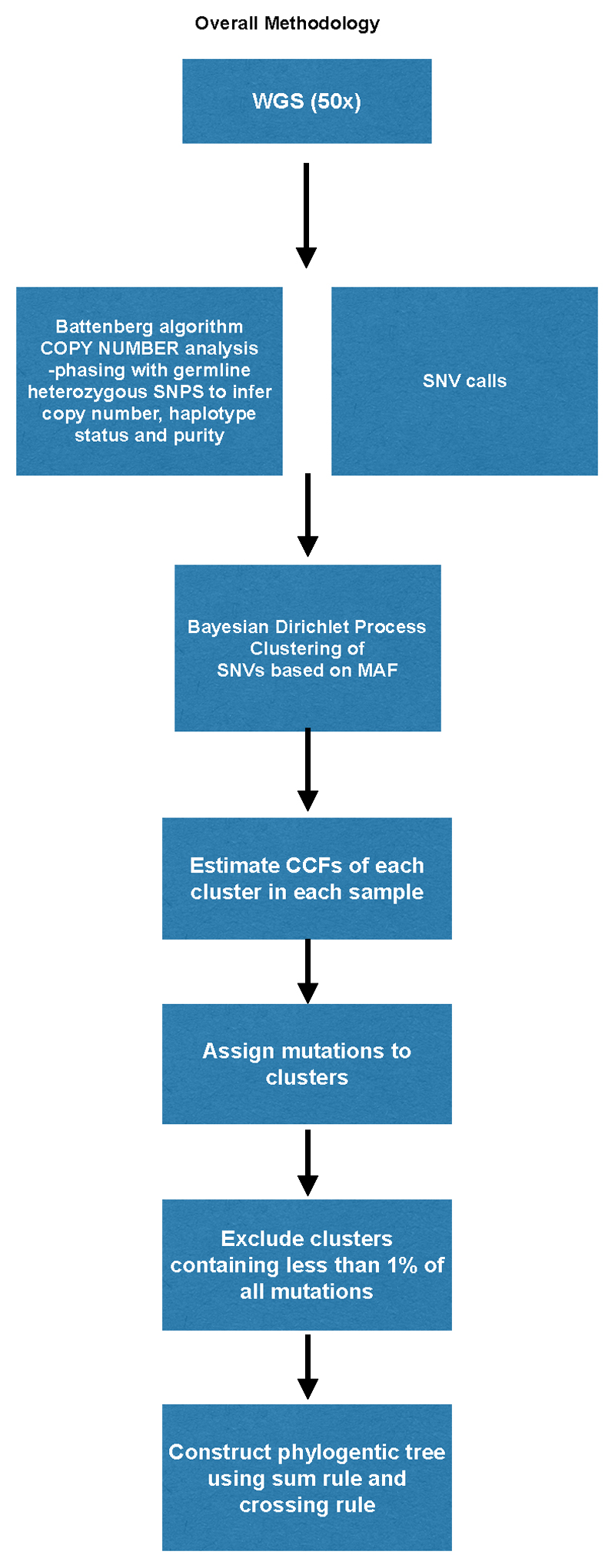
A. The details of phylogenetic tree reconstruction is further elaborated in Supplementary methods, Mutation clustering and phylogenetic tree construction (p.25).

Extended Data Fig. 2. Phylogenetic tree construction for example case S3

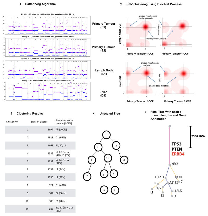
1) Battenberg algorithm to determine total copy number (purple line) and minor allele (blue line). Y-axis =number of chromosome copies, X-axis= chromosome and position. The average ploidy, aberrant cell fraction (cellularity) and goodness of fit to the model are shown for each sample, Primary E1, E2, Lymph node L1 and Distant metastasis D1. The goodness of fit is a measure of the amount of the genome with clonal, rather than subclonal copy number states. D1 has a subclonal mix of different copy number states resulting in noninteger total copy number, for example on chromosome 2, resulting in a goodness of fit below 100%. 2) Bayesian Dirichlet Process to cluster SNVs based on CCF in each sample. The density plots show the posterior probability of a mutational cluster, these are produced for every pair of samples and selected plots are shown High density at CCF of (0,0) indicates subclones that are not present in the pair of samples shown in a particular plot. 3) Clustering of results – Clusters are identified as local maxima in the posterior density. The table shows the number of SNVs assigned to each cluster, and their associated CCFs. 4) Unscaled Tree construction using the sum rule and crossing rule as detailed in Supplementary Methods p25. 5) Final Tree -The tree is drawn as seen in Figures 2 and Extended Data2, branch lengths are proportional to the number of SNVs assigned to each subclone. Scales vary on a per case basis depending on the total number of SNVs, in order to fit cases on one figure. Trees are annotated with the gene names of known drivers, and the colour of each branch represents a trunk (pink), branch (purple) or leaf (yellow). The grey circles represent clones and subclones and their CCFs are shown in Supplementary Table5 and 6.

Extended Data Fig. 3. Phylogenetic trees of cases in cohort with only nodal or distant organ disease, as derived from H-WGS

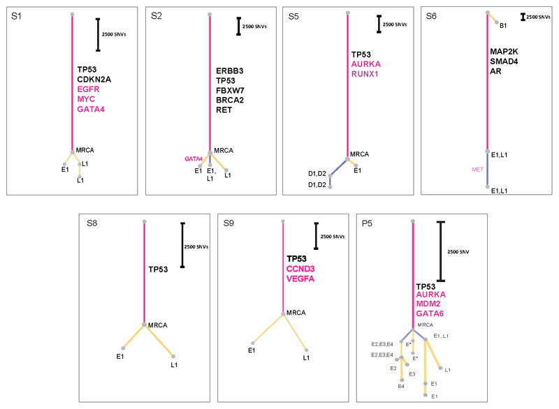
E=esophagus, D=distant organ, L=lymph node, B= Barrett’s. For precise anatomical locations, refer to Supplementary Table3 and 4. MRCA=most recent common ancestor. Pink=trunk (shared events), Purple=branch (shared by more than one sample), Yellow=leaf (unique to one sample). Grey dots at the end of the lines (truncal, branches or leaves) represent subclones or clones, whose CCFs are shown in Supplementary Tables5 and 6. Trees are annotated with key driver events as identified from the literature^,,. Black=point mutations, Red=copy number alterations, purple= structural variants. The adjacent scales are relative to the number of SNVs in that particular case and hence constructed on a case by case basis.

Extended Data Fig. 4. Structural variation of 18 metastatic esophageal adenocarcinoma cases

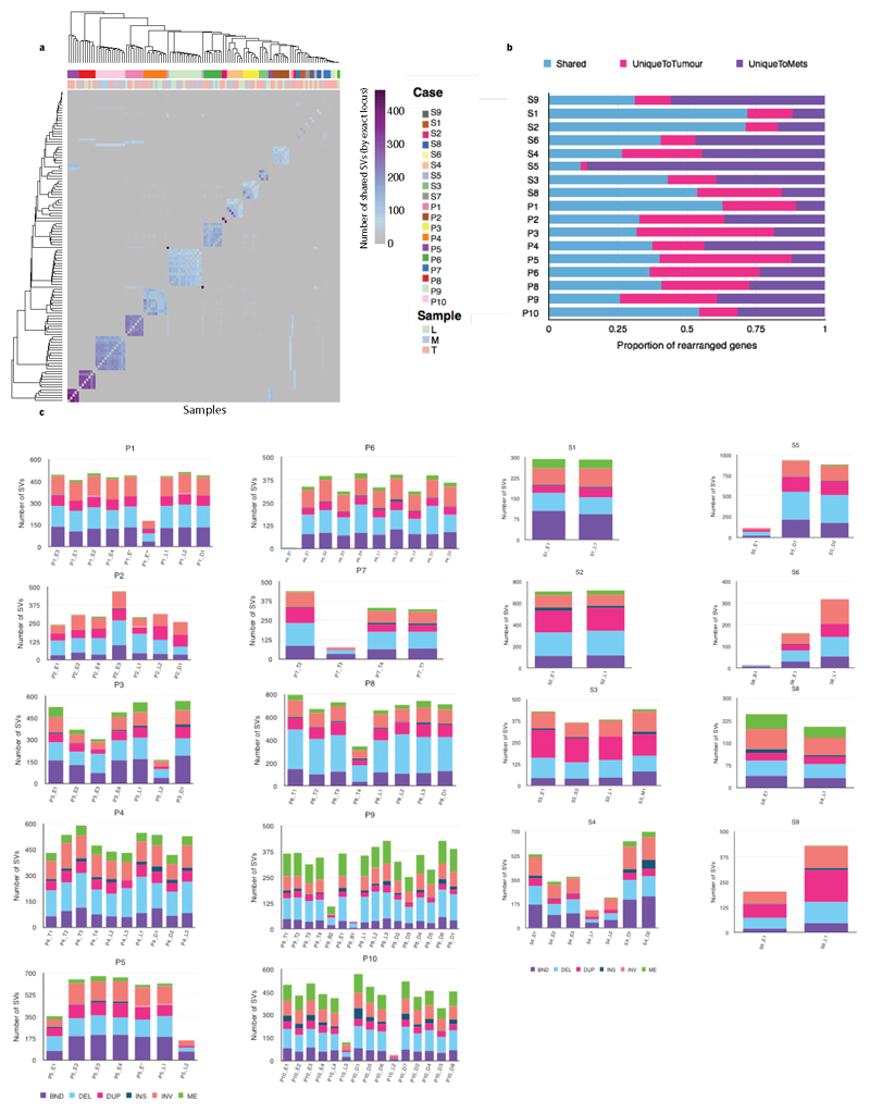
a. Similarity matrix based clustering for all SVs 122 genomes across 19 cases. SVs were deemed to refer to the same rearrangement event across cases if their corresponding breakpoint locations fell within a window of maximum 50 bp. The individual sample types are shown as a separate row on the x axis with the color key depicting the sample type. The purple scale indicates the number of shared SVs. (L=lymph nodes; M=metastasis; T=tumor). b. Histogram showing the percentage of rearranged genes that are concordant, unique to tumors and unique to metastases. Two-tailed Welch test P=0.2674 demonstrating no overall difference between total number of SVs in primary, local lymph nodes and distant metastases c. Stacked bar charts showing the composition of various SVs in each sample on a per patient basis INV= inversion, ME= mobile element, BND= translocation DEL=deletion, DUP=duplication, INS= insertion.

Extended Data Fig. 5. Random simulation model for S-WGS cluster detection

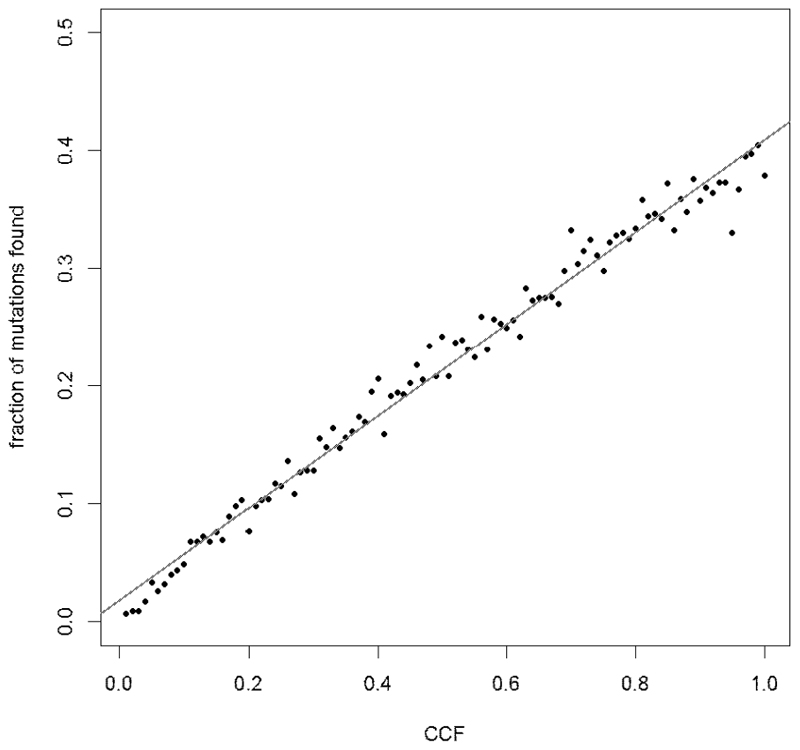
The number of mutations detected correlates strongly with the CCF of the cluster (Pearson r=0.992, n=100). Number of mutations in each cluster =1000.

Extended Data Fig. 6. Correlation of fraction of mutations detected with CCF as a function of cluster size using simulated S-WGS data

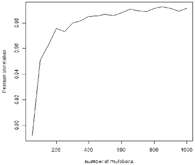
Pearson correlation coefficient is above 0.97 for clusters with 200 or more mutations.

Extended Data Fig. 7. Bar chart demonstrating the Pearson correlation coefficient of VAF at 1xWGS and High Depth Resequencing (n=33)

Extended Data Fig. 8. Detection of Selection in subsets of mutations

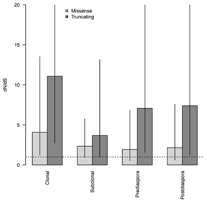
SNVs and indels from all cases (n=18) were aggregated into 4 different subsets: clonal = variants found in the MRCA (n=378453); subclonal = variants not found in the MRCA (n=516136); pre-diaspora = variants found above the diaspora founder clone in the phylogenetic tree (n=313545); post-diaspora = variants found in the diaspora founder or in clones below the founder in the phylogenetic tree (n=295316). Within each subset, dN/dS analysis was performed separately on: missense variants; truncating variants. Bars show maximum likelihood estimates of dN/dS values, with values greater than 1 (dashed line) indicating positive selection. Vertical lines = 95% confidence intervals, estimated using Wald test.

Extended Data Fig. 9. Percentage of truncal and branch clusters in tissue from earlier time-points

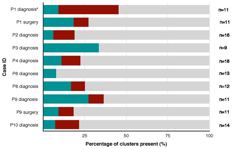
Stacked horizontal bar chart representing the percentage of truncal and branch clusters present in tissue from earlier time-points on the x-axis and the Case ID on the y-axis. P1 diagnosis* is a frozen sample, while the rest are FFPE. Blue = truncal, maroon = branch, grey = not present. The number of clusters (n) is demonstrated for each case.

Extended Data Fig. 10. ctDNA analysis from historical plasma samples

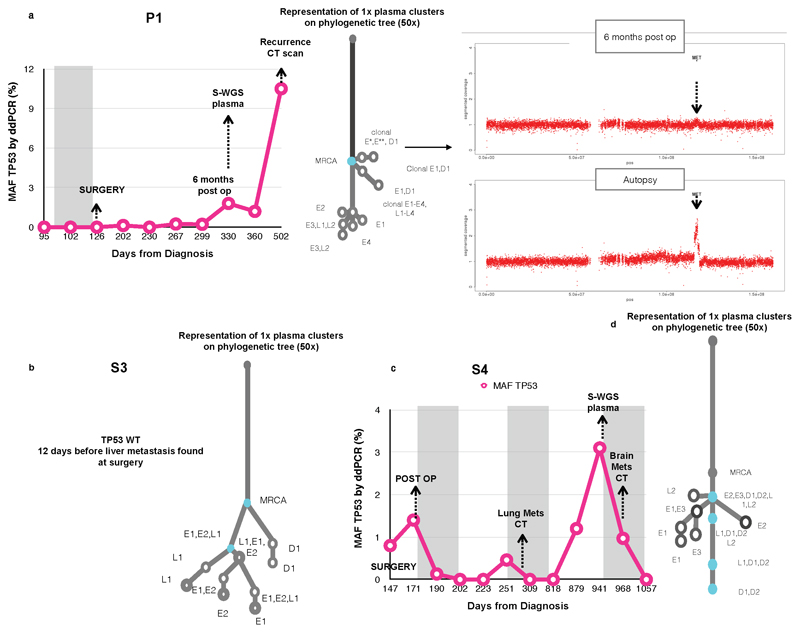
Digital PCR traces of mutant allele fraction for TP53 on the Y-axis and days from diagnosis on the X-axis, and grey areas indicate periods of therapy. Where subclones and clones are seen at 1xWGS on plasma, they are highlighted on the 50x phylogenetic tree (coloured blue). The samples in which these subcloens and clones are present in are shown in Supplementary Table3. There was no TP53 data for S3 as it was wild type for TP53 mutations. Copy number traces for P1 are shown, with the arrow demonstrating an area of MET amplification.

Figure 1. Overall project strategy and study design

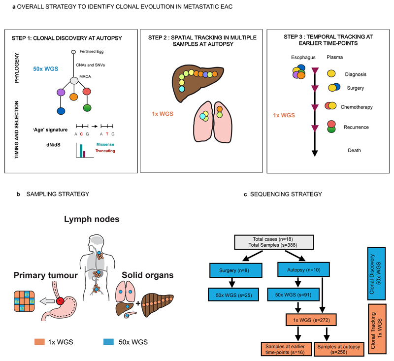
a. Overall Strategy to identify clonal evolution in metastatic EAC. There were three main steps in this study which comprised: Clonal discovery at autopsy (see Supplementary Note High Depth Whole Genome Sequencing (50x WGS), Mutation clustering and phylogenetic tree construction, dN/dS analysis and Mutational Signature Analysis); Spatial tracking at autopsy (see Supplementary Note Shallow Whole Genome Sequencing (1x WGS) and Temporal tracking at earlier time-points (see Supplementary Note Shallow Whole Genome Sequencing (1x) for Subclone identification, Supplementary Table 12 for precise samples for plasma and Extended Data Fig. 9 for FFPE diagnostic samples). Colored circles depict clones and subclones respectively. b. Sampling Strategy at Rapid Autopsy. Areas sampled for the 50x WGS part of the study are shown in blue and for 1x WGS are shown in orange. c. Study Design and Sequencing Strategy. The flow chart demonstrates the study design and how this relates to sequencing. Clonal Discovery is in blue and Clonal Tracking in orange. The sample distribution for 50x WGS and 1x WGS are shown. 50x WGS = High depth WGS (50x), 1x WGS = Shallow WGS (1x). n = number of cases, s = number of samples. †=248 solid tissue samples, and 8 ctDNA at autopsy. CNA, copy number alteration; SNV, single nucleotide variant; MRCA, most recent common ancestor.

Figure 2. Phylogenetic Analysis of ten cases with nodal and distant metastases

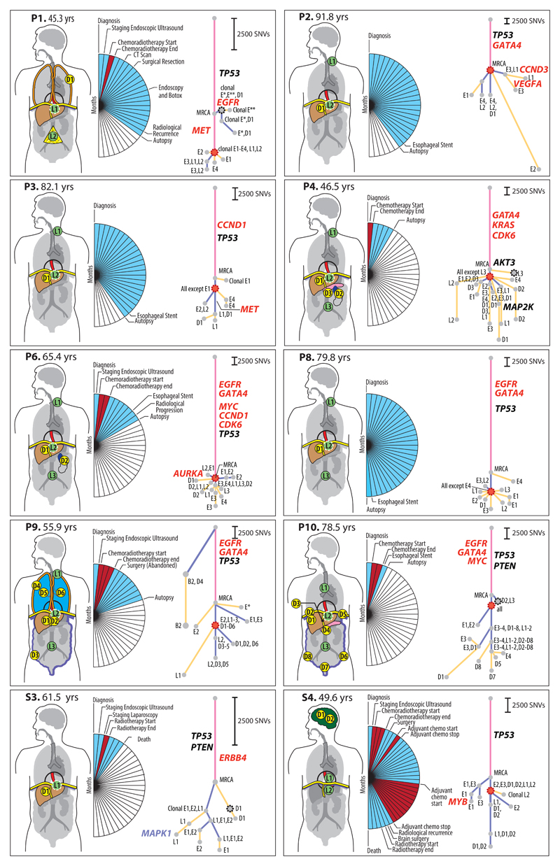
Patient body maps (S=surgical case, P=rapid autopsy) are shown. Green circles denote lymph node metastases and yellow circles distant metastases. The labels within each circle describe the specific location (see Supplementary Table 3, 4). An organ is shown in color if metastases were sequenced from that site. The adjacent wedged semi-circle depicts the clinical timelines for each patient. Each wedge corresponds to one month; blue wedges indicate the total lifetime of the patient and red wedges periods of therapy. Phylogenetic trees for each patient are shown and methodology is in Supplementary Note and Extended Data Fig. 1a-b; pink = truncal events shared by all samples, purple = branch events shared by more than one sample, yellow = leaves, events unique to a sample. The circle at the end of a trunk, branch or leaf represents a clone or subclone. Each clone or subclone is annotated to show which samples it is present in. E1-E4 = primary esophageal tumor, L1-L4= lymph nodes, D1-8 =distant metastases, B = Barrett’s Esophagus. A subclone annotated with E1, L2 for example indicates that this subclone is seen only in samples E1 and L2. The CCF of each subclone/clone (barring the MRCA) is in Supplementary Table 5 and 6. The length of the branches of the tree are reflective of the number of SNVs in the subclone/clone. The scales adjacent to each case are relative, given the variable number of SNVs per case. Trees are annotated with potential driver events, black: missense variants, red: amplifications. Gray dots outlined with a black dashed line denote the first subclone/clone to metastasize that would be classified as non-curative based on anatomical location. Red dots mark the stellate pattern on the phylogenetic tree.

Figure 3. Mutational Signatures

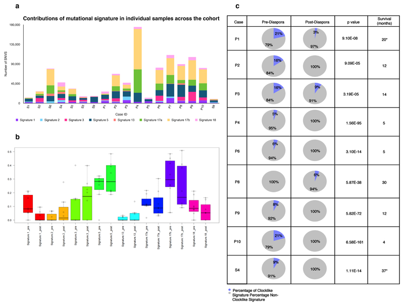
a. Contributions of mutational signature in 18 cases (n=122) across the cohort. The bar chart displays samples on a per case basis (X-axis) and depicts the number of SNVs contributing to each signature (Y-axis). b. Mutational signatures pre-and post-diaspora across all samples (n=122) in 18 cases. Mutations were separately assigned to signatures and the proportion of mutations within each case assigned to each signature is shown. Dark lines = median, Boxes = 25th and 75th quartiles, whiskers extend to the most extreme point within 1.5× interquartile range of the box edge. Signatures 1 mutations have a significantly lower representation in post-diaspora mutations, while signature 3 mutations have significantly high. c. Mutational signature analysis of ageing signature (signature 1) pre-and post-diaspora in all cases (n=8) with local and distant spread (p<1.18 × 10^-90 across all cases) Chi squared test was used to determine the p value. Survival is shown in months from the point of diagnosis *=cases which underwent surgery.

Figure 4. 1x WGS and similarity matrix clustering of 248 further tissue samples from six cases

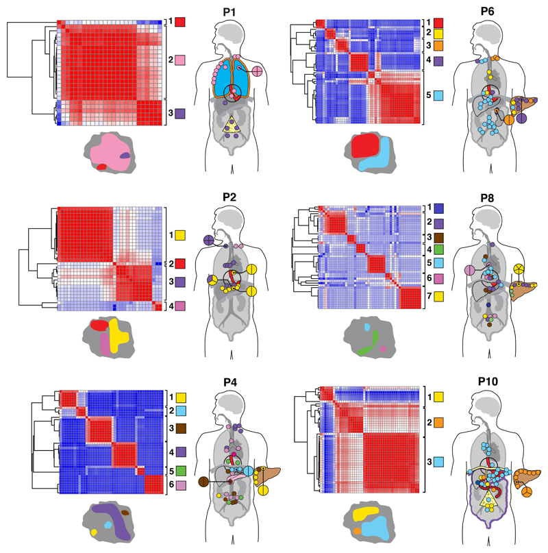
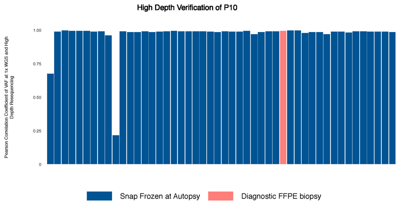
1x WGS was performed at an average depth of 1x to track subclones and clones previously discovered using 50x WGS for further tissue samples (n=248). Pearson correlation similarity matrix clustering was performed on all samples for each case (plotted against each other) with red indicating sample similarity (r=1) and blue indicating dissimilarity (r=-1). Sample sites used in this part of the study are shown in Supplementary Table 9 and the entire organ is highlighted if solid organ sites were sequenced. For example, liver metastases were only seen in P4, P6, P8, P10. Similarly, P2 had lymph nodes only (only colored dots are seen which represent lymph nodes, no solid organs are highlighted). Clustering was performed based on the presence of subclones and clones already detected using 50x WGS and distinct clusters were identified for each case as demonstrated by the adjacent key per case (each group is both colored and numbered). Samples are displayed on the adjoining body maps for which the color coding corresponds to the genomic clustering in the adjacent heatmap. Sites with multiple samples are magnified and the division of samples shown. Maps of the primary tumor with representation of metastatic subclones are shown with each case, with the colors of the subclones being the same as those in the matrix and body map. Areas shaded red in the primary tumor represent subclones that were not detected in the metastatic samples that underwent 1x WGS and were instead confined to areas of the primary tumor.

Figure 5. Temporal and spatial tracing of metastatic subclones in plasma

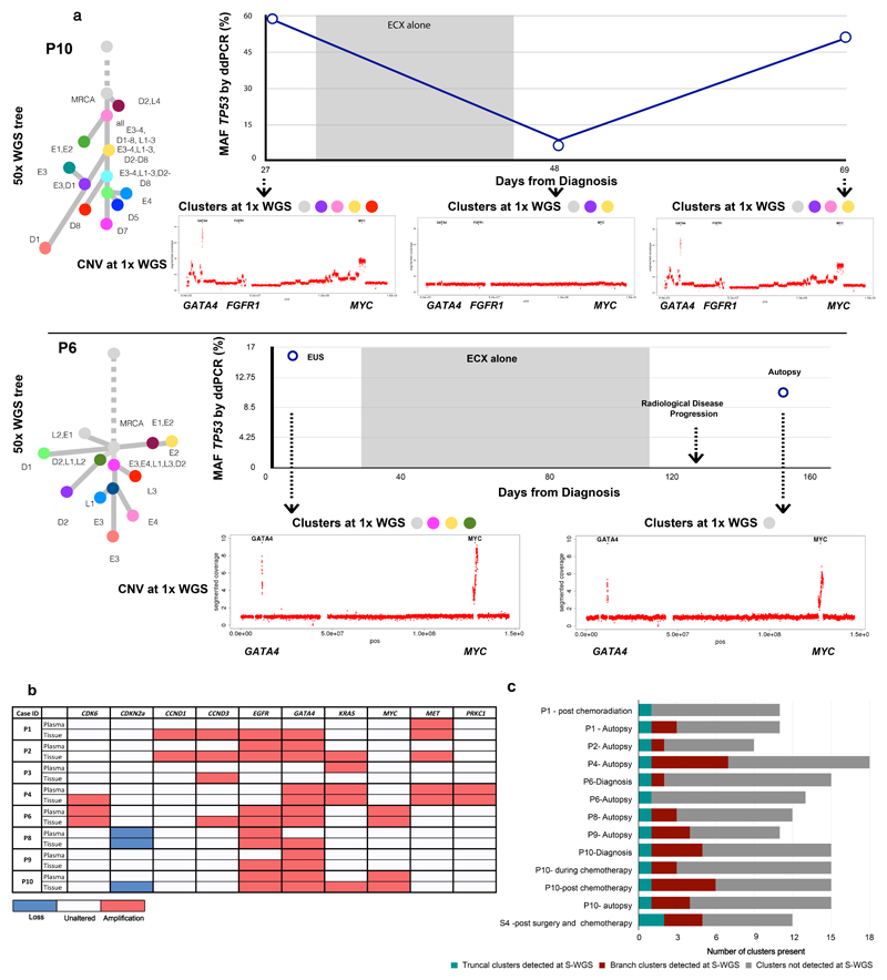
a. Plasma ctDNA 1x WGS and digital droplet PCR (ddPCR) analysis for TP53 mutant allele fraction (MAF) for P10 and P6. The MAF of TP53 (%) is shown on the Y-axis and days from diagnosis are shown on the X-axis. The shaded areas represent time periods of therapy. 1x WGS at select time-points was performed and the clonal composition of these samples are shown by the presence of colored clusters. The color of each corresponds to the color of the corresponding node on the adjacent 50x phylogenetic tree with the presence of colored clusters which correlate with the 50x tree. Moreover, copy number traces for each time point are shown for select chromosomes. b. The presence or absence of amplifications and deletions in plasma compared to tissue, detected from 1x WGS for 8 cases. Tissue refers to all samples collected at autopsy and at earlier time-points. c. Stacked bar charts to demonstrate the presence or absence of clusters across all plasma samples, including truncal and branch clusters using 1x WGS.

Figure 6. Diaspora model of metastatic spread and associated features

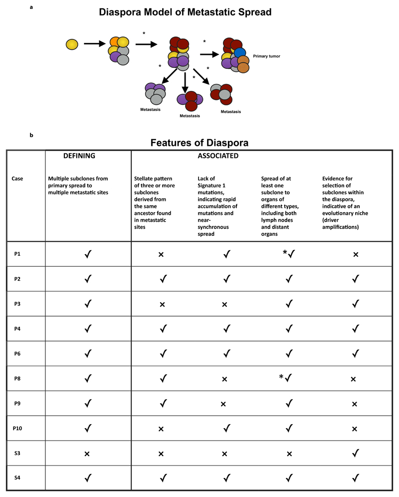
Panel a depicts clonal diaspora with colored circles representing clones and subclones. *= evidence of selection. Panel b explains the five features seen in diaspora (one is defining, and the other are associated with diaspora) and whether these are present (✓) or absent (x) in each case. *✓ implies that the feature is present, and that the evidence was from 1x WGS.