Machine-learned patterns suggest that diversification drives economic development

Abstract

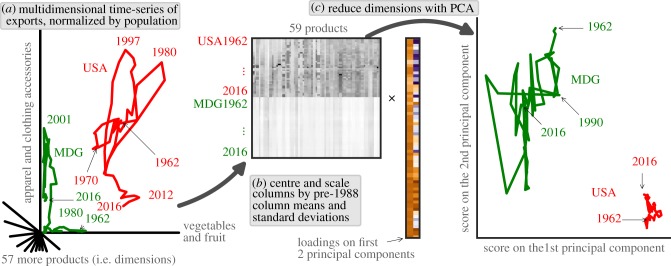
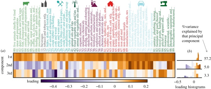
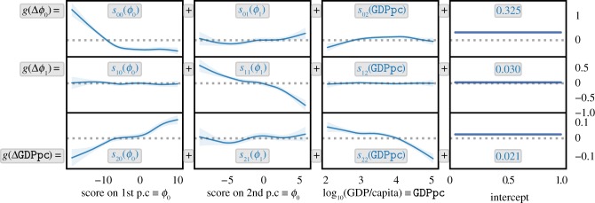
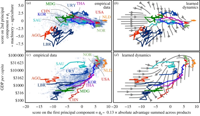
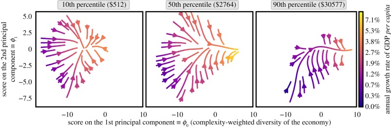
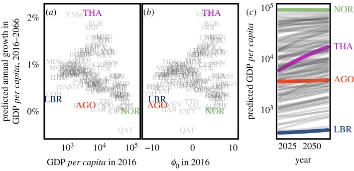
We combine a sequence of machine-learning techniques, together called Principal Smooth-Dynamics Analysis (PriSDA), to identify patterns in the dynamics of complex systems. Here, we deploy this method on the task of automating the development of new theory of economic growth. Traditionally, economic growth is modelled with a few aggregate quantities derived from simplified theoretical models. PriSDA, by contrast, identifies important quantities. Applied to 55 years of data on countries' exports, PriSDA finds that what most distinguishes countries' export baskets is their diversity, with extra weight assigned to more sophisticated products. The weights are consistent with previous measures of product complexity. The second dimension of variation is proficiency in machinery relative to agriculture. PriSDA then infers the dynamics of these two quantities and of per capita income. The inferred model predicts that diversification drives growth in income, that diversified middle-income countries will grow the fastest, and that countries will converge onto intermediate levels of income and specialization. PriSDA is generalizable and may illuminate dynamics of elusive quantities such as diversity and complexity in other natural and social systems.

Keywords: complex systems; dynamical systems; economic development; modelling; non-parametric regression; statistical learning.

Figure 1.

Preprocessing and reducing dimensions of export baskets. (a) Begin with time series of export values of 59 product categories, normalized by population (electronic supplementary material, Eq. (SM-1)) and logarithmically transformed (electronic supplementary material, Eq. (SM-5)) to make large and small countries comparable. For illustration, we show the trajectories of the United States (USA) and Madagascar (MDG). We are illustrating two dimensions here, but in reality the red and green curves live in 59 dimensions. (b) Centre and scale columns by their pre-1988 means and standard deviations. (c) Reduce dimensions with principal components analysis (PCA). Each country’s score in a given principal component represents a certain linear combination of its export basket. Together, the scores on the first few principal components summarize the country’s export basket with just a few numbers. (Online version in colour.)

Figure 2.

The first three principal components are approximately (1) total absolute advantage summed across all products (with more weight on product codes above 50), (2) machinery minus agriculture, and (3) textiles and fertilizer minus coffee and cork. In plot (a), the rows are principal components, the columns are products, and the rectangles’ colours represent the loading (or ‘weight’) of that principal component on that product. The first component loads positively on all products. Thus, what distinguishes countries, above all, is their ‘diversification’ across products. The second component loads highly on machinery (product codes beginning with 7) and other manufactured goods, and it loads negatively on agricultural products. Thus, the direction in 59-dimensional product space orthogonal to the first component that most spreads out observations points towards machinery and away from agriculture. The third component loads positively on clothing and textile products and negatively on cork and wood (24) and coffee, tea and spices (07). The plots labelled (b) are histograms of loadings, across all 59 products, in the corresponding rows. (Online version in colour.)

Figure 3.

Export baskets tend to diversify and converge to a balance of agriculture and manufactured goods. Shown are partial dependence plots of the three equations in (1.2). Each blue (solid) curve is an additive contribution to the quantity written in black on the left-hand side of this figure, which is a link function g applied to the expected yearly change in one of the three variables ϕ₀, ϕ₁, $\mathtt{G}\mathtt{D}\mathtt{P}\mathtt{p}\mathtt{c}$. (See the text after (1.2) for the definition of g.) In each plot, the quantity being plotted is written in blue within the plot. Adding the blue expressions across a row gives the right-hand sides of (1.2). The shaded regions show the 95% CI. Each equation has an intercept, c_i, shown in the right column. The plots on the diagonal have negative trends, suggesting convergence. Interestingly, income is not associated with changes in export baskets, but ϕ₀ appears to drive $\mathtt{G}\mathtt{D}\mathtt{P}\mathtt{p}\mathtt{c}$: diversifying precedes income growth. (Replacing ϕ₀ with diversification preserves the positive trend in the bottom-left plot, but replacing it with per capita exports greatly weakens that relationship; see electronic supplementary material, Figs. SM-13 and SM-14.) (Online version in colour.)

Figure 4.

The learned dynamics (1.2) predict that countries are converging. The left column shows empirical data with blue dots; the right column shows predictions of the model (1.2) as stream plots. The empirical trajectories of eight countries over years 1962–2016 are superimposed on all four plots. Trajectories are labelled at the first available sample (year 1985 for Angola, 1962 for the rest). A country is represented by a triple $({\varphi }_0,{\varphi }_1,\mathtt{G}\mathtt{D}\mathtt{P}\mathtt{p}\mathtt{c})$, and the model (1.2) has been trained on this three-dimensional space, but here we show projections onto (ϕ₀, ϕ₁) in the top row and onto $({\varphi }_0,\mathtt{G}\mathtt{D}\mathtt{P}\mathtt{p}\mathtt{c})$ in the bottom row. (a) Countries tend to diversify (increase ϕ₀) and strike a balance between machinery and agriculture (ϕ₁ ≈ 0). (c) Development success stories (e.g. THA, KOR, CHN) share a common trajectory of increasing ϕ₀ and income. (d) Poor countries may follow in their footsteps, but income in the richest countries may stagnate or even fall. Countries are labelled with United Nations ISO-alpha3 codes. (Online version in colour.)

Figure 5.

Inferred dynamics of export baskets, at three levels of per capita income, predict convergence in the long run. The streamlines show how a country’s export basket, described by its scores (ϕ₀, ϕ₁) on the first two principal components, changes over time according to the GAM (1.2). From left to right, the plots correspond to GDP per capita at the 10th, 50th and 90th percentiles of per capita income among countries in the year 1988. Those percentiles are the value inserted into (1.2); we show streamlines at (ϕ₀, ϕ₁) pairs in the convex hull of all empirical samples $({\varphi }_0,{\varphi }_1,\mathtt{G}\mathtt{D}\mathtt{P}\mathtt{p}\mathtt{c})$ with $\mathtt{G}\mathtt{D}\mathtt{P}\mathtt{p}\mathtt{c}$ within 15% of the value shown at the top of the plot. The predicted yearly change in per capita income is plotted in colour. The model predicts that poor countries move towards a balance of agriculture and machinery before increasing their total exports. (Said formally, ϕ₁ → 0 in the left plot, and ϕ₀ increases substantially in the middle and right plots.) Eventually, all countries are predicted to become rich and to have diverse export baskets (high ϕ₀) that balance between agriculture and machinery (ϕ₁ ≈ 0). (Online version in colour.)

Figure 6.

Catch-up of the diverse, middle-income countries. Shown are predicted annual growth rates of per capita income (in constant 2010 USD per person per year) over the next 50 years as a function of (a) current per capita income and (b) current score ϕ₀ on the first principal component. (c) Predicted trajectories of per capita income. Highlighted are four countries representative of four groups: low-income countries predicted to grow little (Liberia, LBR); middle-income countries with high diversity (high ϕ₀) today predicted to grow a lot (Thailand, THA); middle-income countries with low diversity (low ϕ₀) predicted to grow little (Angola, AGO); and high-income countries predicted to grow little (Norway, NOR). The GAM (1.2) predicts the highest growth in income for economies that currently have intermediate income (annual growth $\approx 1.5\text{\%}$ to 2% for countries with yearly per capita income between $1000 and $20 000) and lower growth rates for poorest countries (0 to 1% growth) and the richest countries (0 to 0.5% growth). (Online version in colour.)

References

1. Voosen P. 2017. How AI detectives are cracking open the black box of deep learning. Science. (10.1126/science.aan7059) - DOI
1. Bongard J, Lipson H. 2007. Automated reverse engineering of nonlinear dynamical systems. Proc. Natl Acad. Sci. USA 104, 9943–9948. (10.1073/pnas.0609476104) - DOI - PMC - PubMed
1. Schmidt M, Lipson H. 2009. Distilling free-form natural laws from experimental data. Science 324, 81–85. (10.1126/science.1165893) - DOI - PubMed
1. Daniels BC, Nemenman I. 2015. Automated adaptive inference of phenomenological dynamical models. Nat. Commun. 6, 8133 (10.1038/ncomms9133) - DOI - PMC - PubMed
1. Zhang L, Li K. 2015. Forward and backward least angle regression for nonlinear system identification. Automatica 53, 94–102. (10.1016/j.automatica.2014.12.010) - DOI
Publication types
LinkOut - more resources