Comparative Study
. 2019 Dec 10:13:75.
doi: 10.3389/fncir.2019.00075. eCollection 2019.

A Comparison of Neural Decoding Methods and Population Coding Across Thalamo-Cortical Head Direction Cells

Affiliations
Comparative Study

A Comparison of Neural Decoding Methods and Population Coding Across Thalamo-Cortical Head Direction Cells

Zishen Xu et al. Front Neural Circuits. .

Abstract

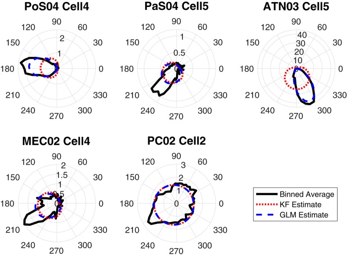
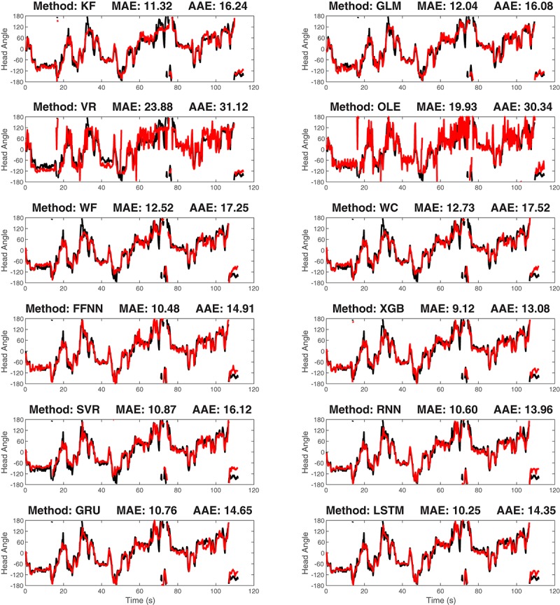
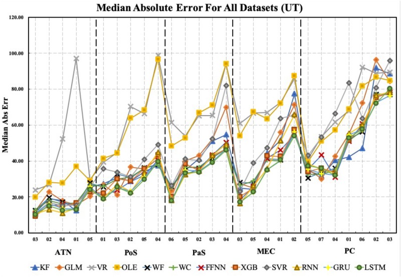
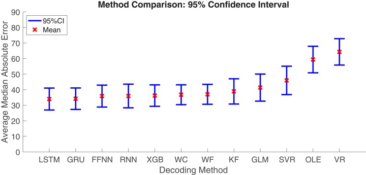
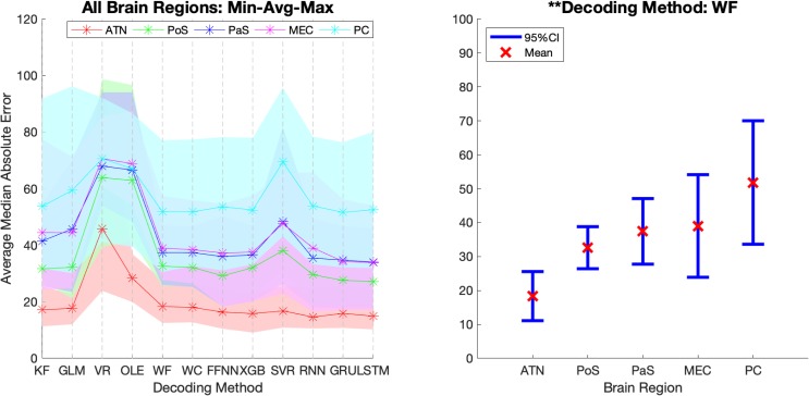
Head direction (HD) cells, which fire action potentials whenever an animal points its head in a particular direction, are thought to subserve the animal's sense of spatial orientation. HD cells are found prominently in several thalamo-cortical regions including anterior thalamic nuclei, postsubiculum, medial entorhinal cortex, parasubiculum, and the parietal cortex. While a number of methods in neural decoding have been developed to assess the dynamics of spatial signals within thalamo-cortical regions, studies conducting a quantitative comparison of machine learning and statistical model-based decoding methods on HD cell activity are currently lacking. Here, we compare statistical model-based and machine learning approaches by assessing decoding accuracy and evaluate variables that contribute to population coding across thalamo-cortical HD cells.

Keywords: anterior thalamus; memory; navigation; parahippocampal; parietal; spatial behavior.


Figures

FIGURE 1
FIGURE 1
Graphic representation of the Kalman Filter and Generalized Linear Model: The main model is a hidden Markov chain structure. HDs follow a Markov chain and spike counts at the current time bin are independent from the counts from previous time bins.
FIGURE 2
FIGURE 2
Illustration of the coverage of the full range of HDs: If all the preferred direction vectors cover only half of the possible HDs, then the vectors in the other half circle cannot be achieved by a non-negative weighted linear combination of these vectors, so the predicted angles will not cover all values between 0° and 360°.
FIGURE 3
FIGURE 3
The structure of feedforward neural network and Recurrent Neural Network (RNN): Top: The typical structure of a feedforward neural network. Each unit will calculate a weighted sum of the units in the previous layer that connect to it by an arrow. Then by adding an intercept term and transforming the value by an activation function, the unit obtains the value it sends out. Bottom: the structure of a Recurrent Neural Network component. The input vectors are connected by a chain hidden layer. Each hidden unit is the transformed value of the linear combination of the corresponding input unit and previous hidden unit. The last hidden unit value (vector) will be transformed by another non-linear function and sent to the dense layer to compute the output.
FIGURE 4
FIGURE 4
The structure of Gated Recurrent Unit and Long Short-Term Memory units: Left: this is the structure of the Gated Recurrent Unit (GRU). The “update gate” zt is used to determine if the update h~t will be applied to ht. rt is the “reset gate” and is used to determine if the previous hidden value (also the output value) ht1 will be kept in the memory. The effects of the two gates are achieved by sigmoid activation functions which can be learned during training. Right: The structure of the Long Short-Term Memory (LSTM) unit. LSTM is complex and includes one more hidden value Ct and more gates compared to GRU. Each gate can be seen in the plot where the σ sign appears (i.e., sigmoid activation function). The first σ is the “forget gate” which controls whether previous hidden value, Ctv will be used to calculate current output and kept in the memory. The second σ is the “input gate” which controls whether the new input will be used to calculate current output. The third σ is the “output gate” which filters the output, i.e., controls what part of the output values to send out as ht.
FIGURE 5
FIGURE 5
The true-vs.-estimated tuning plots in 6-degree bins for one HD cell in each brain region: The polar plots show firing rates vs. HD. The black curves are the true tuning functions, smoothed by a Gaussian kernel function. The red curves are the estimated functions using the Kalman Filter (KF) method and the blue curves are the estimated functions using the Generalized Linear Model (GLM) method.
FIGURE 6
FIGURE 6
The true-vs.-predicted head angle plotted as a function of time for a representative ATN dataset for each of the 12 decoding methods: The black curves are the true curves and the red curves are the predicted curves. Test data is shown. Predicted curves are constructed using a model generated from a separate training segment of the data. The method name and decoding accuracy measured as median absolute error (MAE) are shown on the title of each plot (average absolute error, AAE, is also shown). KF, Kalman Filter; GLM, Generalized Linear Model; VR, Vector Reconstruction; OLE, Optimal Linear Estimator; WF, Wiener Filte, and WC, Wiener Cascade. The remaining six are machine learning methods: SVR, Support Vector Regression; XGB, XGBoost; FFNN, Feedforward Neural Network; RNN, Recurrent Neural Network; GRU, Gated Recurrent Unit; LSTM, Long Short-Term Memory.
FIGURE 7
FIGURE 7
The median absolute error is shown for each brain region, each dataset, and each decoding method. Datasets for each brain region are sorted from lowest to highest median absolute error (i.e., from best to worst decoding accuracy). Note that median absolute error varies considerably within regions and on average increases from ATN to parahippocampal and PC regions. KF, Kalman Filter; GLM, Generalized Linear Model; VR, Vector Reconstruction; OLE, Optimal Linear Estimator; WF, Wiener Filter; WC, Wiener Cascade; SVR, Support Vector Regression; XGB, XGBoost; FFNN, Feedforward Neural Network; RNN, Recurrent Neural Network; GRU, Gated Recurrent Unit; LSTM, Long Short-Term Memory.
FIGURE 8
FIGURE 8
Mean ± 95% Confidence-Interval (CI) Median Absolute Error (MAE) for each decoding method. Data from different brain regions and datasets were pooled. KF, Kalman Filter; GLM, Generalized Linear Model; VR, Vector Reconstruction; OLE, Optimal Linear Estimator; WF, Wiener Filter; WC, Wiener Cascade; SVR, Support Vector Regression; XGB, XGBoost; FFNN, Feedforward Neural Network; RNN, Recurrent Neural Network; GRU, Gated Recurrent Unit; LSTM, Long Short-Term Memory.
FIGURE 9
FIGURE 9
Decoding accuracy varies across brain regions. The average Median Absolute Error (MAE) for each area and each decoding method. The shading in the left panel represents the range of the MAE values while the error bars in the right panel represents the 95% Confidence-intervals of the average MAE values for a representative decoding method. 95% Confidence-interval plots for the remaining 11 methods are shown in Supplementary Material S10. KF, Kalman Filter; GLM, Generalized Linear Model; VR, Vector Reconstruction; OLE, Optimal Linear Estimator; WF, Wiener Filter; WC, Wiener Cascade; SVR, Support Vector Regression; XGB, XGBoost; FFNN, Feedforward Neural Network; RNN, Recurrent Neural Network; GRU, Gated Recurrent Unit; LSTM, Long Short-Term Memory; ATN, Anterior Thalamic Nuclei; PoS, Postsubiculum; PaS, Parasubiculum; MEC, Medial Entorhinal Cortex; PC, Parietal Cortex. ∗∗p < 0.01.
FIGURE 10
FIGURE 10
Scatterplots of median absolute error vs. number of cells for all 12 methods. The dashed line is the fitted linear regression. The correlation coefficient (r) and the corresponding p-value are shown on the top-right corner of each panel. The significance levels are shown with symbols on the top-left corner ∗∗∗p < 0.001; ∗∗p < 0.01; p < 0.05. KF, Kalman Filter; GLM, Generalized Linear Model; VR, Vector Reconstruction; OLE, Optimal Linear Estimator; WF, Wiener Filter; WC, Wiener Cascade; SVR, Support Vector Regression; XGB, XGBoost; FFNN, Feedforward Neural Network; RNN, Recurrent Neural Network; GRU, Gated Recurrent Unit; LSTM, Long Short-Term Memory.
FIGURE 11
FIGURE 11
Tuning influences decoding accuracy. Top Row. Examples illustrating the relationship between scaled standard deviation (scaled STD) and tuning for single cells from ATN (left), PoS (middle), and MEC (right). The plots of tuning curves were smoothed by a Gaussian kernel function. The scaled STD is computed by taking standard deviation of the scaled (divided by maximum) firing rate. Bottom 4 Rows. Linear regression data is shown for each decoding method as a function of scaled STD (i.e., indicator of tuning strength). One cell was randomly selected from each dataset to avoid repeatedly sampling the same decoding score. ∗∗∗p < 0.001; ∗∗p < 0.01.
FIGURE 12
FIGURE 12
Example histograms of spike counts (top three, bottom left and bottom middle), and an example Median Absolute Error (MAE) vs. response rate scatterplot (bottom right): The dataset’s label and response rate are listed in the title. The example scatterplot illustrates the modest relationship between response rate and decoding accuracy. Scatterplots for all the 12 methods are shown in Supplementary Material S12. The dashed line in the scatterplot is the fitted linear regression. Optimal Linear Estimator (OLE).

Similar articles

Cited by

References

    1. Bassett J. P., Wills T. J., Cacucci F. (2018). Self-organized attractor dynamics in the developing head direction circuit. Curr. Biol. 28 609–615. 10.1016/j.cub.2018.01.010 - DOI - PMC - PubMed
    1. Berens P. (2009). CircStat: a MATLAB toolbox for circular statistics. J. Stat. Softw. 31 1–21.
    1. Blair H. T., Sharp P. E. (1995). Anticipatory head direction signals in anterior thalamus: evidence for a thalamocortical circuit that integrates angular head motion to compute head direction. J. Neurosci. 15 6260–6270. 10.1523/jneurosci.15-09-06260.1995 - DOI - PMC - PubMed
    1. Boccara C. N., Sargolini F., Thoresen V. H., Solstad T., Witter M. P., Moser E. I. (2010). Grid cells in pre- and parasubiculum. Nat. Neurosci. 13 987–994. 10.1038/nn.2602 - DOI - PubMed
    1. Butler W. N., Taube J. S. (2017). Oscillatory synchrony between head direction cells recorded bilaterally in the anterodorsal thalamic nuclei. J. Neurophysiol. 117 1847–1852. 10.1152/jn.00881.2016 - DOI - PMC - PubMed

Publication types

LinkOut - more resources