OpenSFDI: an open-source guide for constructing a spatial frequency domain imaging system

Abstract

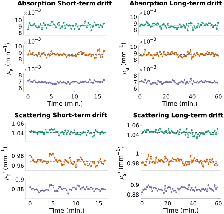
Significance: Spatial frequency domain imaging (SFDI) is a diffuse optical measurement technique that can quantify tissue optical absorption (μ_a) and reduced scattering (<inline-formula>${\mu }_s^{\text{'}}$</inline-formula>) on a pixel-by-pixel basis. Measurements of μ_a at different wavelengths enable the extraction of molar concentrations of tissue chromophores over a wide field, providing a noncontact and label-free means to assess tissue viability, oxygenation, microarchitecture, and molecular content. We present here openSFDI: an open-source guide for building a low-cost, small-footprint, three-wavelength SFDI system capable of quantifying μ_a and <inline-formula>${\mu }_s^{\text{'}}$</inline-formula> as well as oxyhemoglobin and deoxyhemoglobin concentrations in biological tissue. The companion website provides a complete parts list along with detailed instructions for assembling the openSFDI system.<p> Aim: We describe the design of openSFDI and report on the accuracy and precision of optical property extractions for three different systems fabricated according to the instructions on the openSFDI website.</p> <p> Approach: Accuracy was assessed by measuring nine tissue-simulating optical phantoms with a physiologically relevant range of μ_a and <inline-formula>${\mu }_s^{\text{'}}$</inline-formula> with the openSFDI systems and a commercial SFDI device. Precision was assessed by repeatedly measuring the same phantom over 1 h.</p> <p> Results: The openSFDI systems had an error of 0 ± 6 % in μ_a and -2 ± 3 % in <inline-formula>${\mu }_s^{\text{'}}$</inline-formula>, compared to a commercial SFDI system. Bland-Altman analysis revealed the limits of agreement between the two systems to be ± 0.004 mm ^{- 1} for μ_a and -0.06 to 0.1 mm ^{- 1} for <inline-formula>${\mu }_s^{\text{'}}$</inline-formula>. The openSFDI system had low drift with an average standard deviation of 0.0007 mm ^{- 1} and 0.05 mm ^{- 1} in μ_a and <inline-formula>${\mu }_s^{\text{'}}$</inline-formula>, respectively.</p>,<p> Conclusion: The openSFDI provides a customizable hardware platform for research groups seeking to utilize SFDI for quantitative diffuse optical imaging.</p>

Keywords: diffuse optics; frequency domain; modulated imaging; open source; optical properties; spatial frequency domain imaging.

Fig. 1

Schematic representation of the openSFDI system. CL, collimating lens; DCM, dichroic mirror; AL, achromatic lens; P, linear polarizers; M, mirror; C, camera; DMD, digital micromirror device.

Fig. 2

CAD rendering of the openSFDI system with the light paths for the three wavelengths. L, light-emitting diode; CL, collimating lens (only one of three labeled); DCM, dichroic mirror (only one of two indicated); ACL, achromatic lens; P, linear polarizers; M, mirror; C, camera; DMD, digital micromirror device.

Fig. 3

OpenSFDI results in biological tissue. (a) Diffuse reflectance of the back of a hand at 865 nm. Superficial vasculature is apparent due to hemoglobin absorption. Boxes indicate regions of interest for the line plots. (b) Estimated concentration of oxyhemoglobin. (c) Estimated concentration of deoxyhemoglobin. (e) Image of ${\mu }_s^{\prime }$ at 865 nm. (f) Absorption spectra (points) and chromophore fits for the vascular compartment (red solid line) and nonvascular compartment (blue dashed line). (g) Scattering spectra (points) and power law fits (lines) for the vascular and nonvascular compartments. Error bars represent $\pm 1$ standard deviation of the pixels in the regions of interest. Scale bar applies to all images.

Fig. 4

Accuracy of three openSFDI systems compared with a commercial SFDI device. Data points represent the average optical property of a phantom measured three times. Error bars are the standard deviation across the three measurements. System 1 was constructed at Boston University and used an FLIR CMOS camera. System 2 was constructed at Boston University and used an Andor sCMOS camera. System 3 was constructed at the University of Maine and used a Thorlabs sCMOS camera. The average ± standard deviation difference between openSFDI and the commercial system was $0\pm 6\%$, $4\pm 6\%$, and $-7\pm 15\%$ for ${\mu }_a$ and $-2\pm 3\%$, $-1\pm 4\%$, and $1\pm 6\%$ for ${\mu }_s^{\prime }$, respectively. Note that each system uses slightly different wavelengths due to variations in LED manufacturing. Error bars on the bottom plots are similar in size to the data points.

Fig. 5

Bland–Altman plots comparing openSFDI (OS) with a commercial, gold standard (GS), SFDI system. The horizontal axis is the average of the two instruments, while the vertical axis is the difference between the two. The solid horizontal line is the average difference and the dashed horizontal lines show estimates of the limits of agreement. Error bars on those lines indicate uncertainty surrounding those estimates. The average difference between the two devices was $1.5\times {10}^{-4}{\mathrm{mm}}^{-1}$ in ${\mu }_a$ and $0.017{\mathrm{mm}}^{-1}$ in ${\mu }_s^{\prime }$, respectively. The limits of agreement in ${\mu }_a$ and ${\mu }_s^{\prime }$ were $-0.0038$ and $0.0041\pm 0.0007$ and $-0.06$ and $0.09\pm 0.02$, respectively.

Fig. 6

Results from a 15-min drift measurement (left column) and a 60-min drift measurement (right column) showing the stability of the ${\mu }_a$ (top row) and ${\mu }_s^{\prime }$ (bottom row) measurements. The subplots in each panel correspond to the different wavelengths with the top plot representing 660 nm, the middle plot representing 735 nm, and the bottom plot representing 865 nm. Dashed lines represent the means of each measurement. The average standard deviation of ${\mu }_a$ was $0.0004{\mathrm{mm}}^{-1}$ and the average standard deviation of ${\mu }_s^{\prime }$ was 0.005.

Fig. 7

(a) Raw intensity image of a 1.75-cm-diameter hemispheric phantom showing how the intensity changes as a function of height. (b) Wrapped phase image of the same phantom. The effect of height can be clearly seen by the curve of the phase isolines. (c) Three-dimensional rendering of the object’s profile following phase unwrapping and calibration of panel (b).