A distributional code for value in dopamine-based reinforcement learning

Abstract

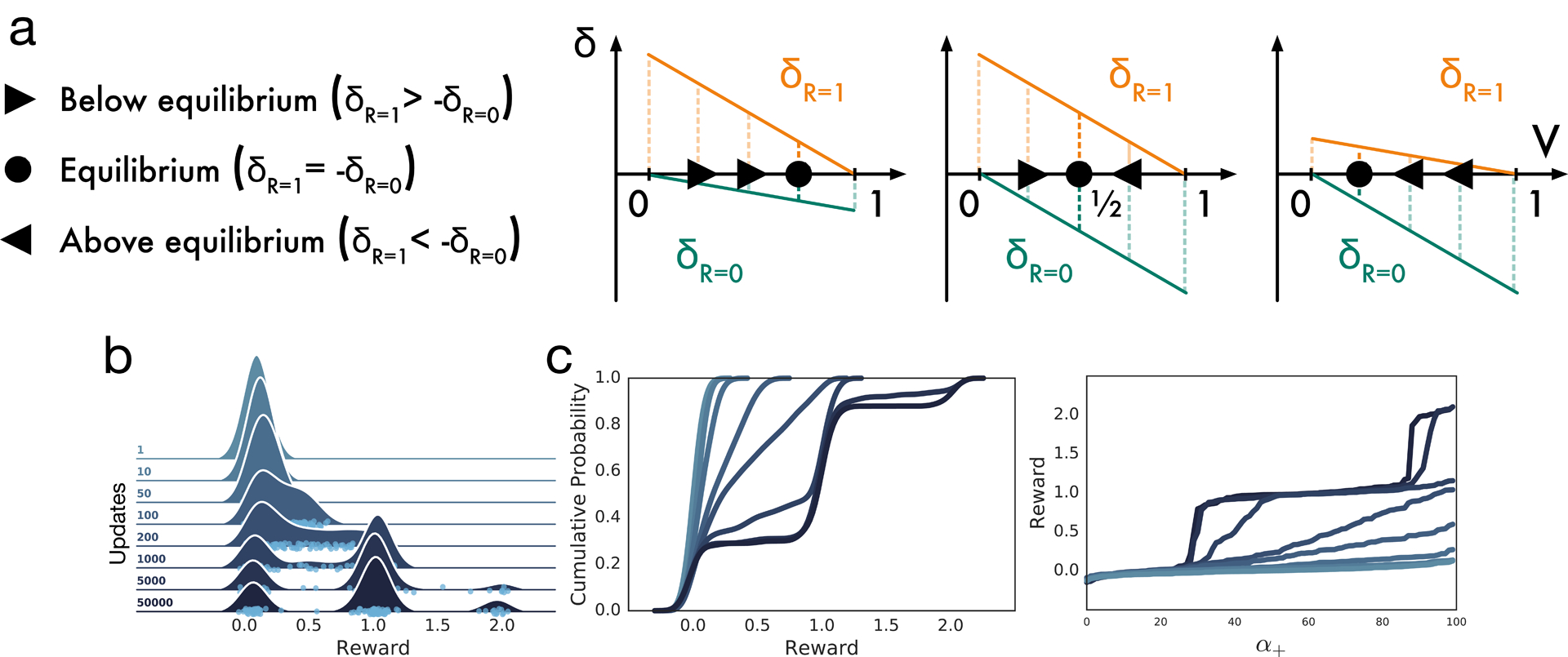
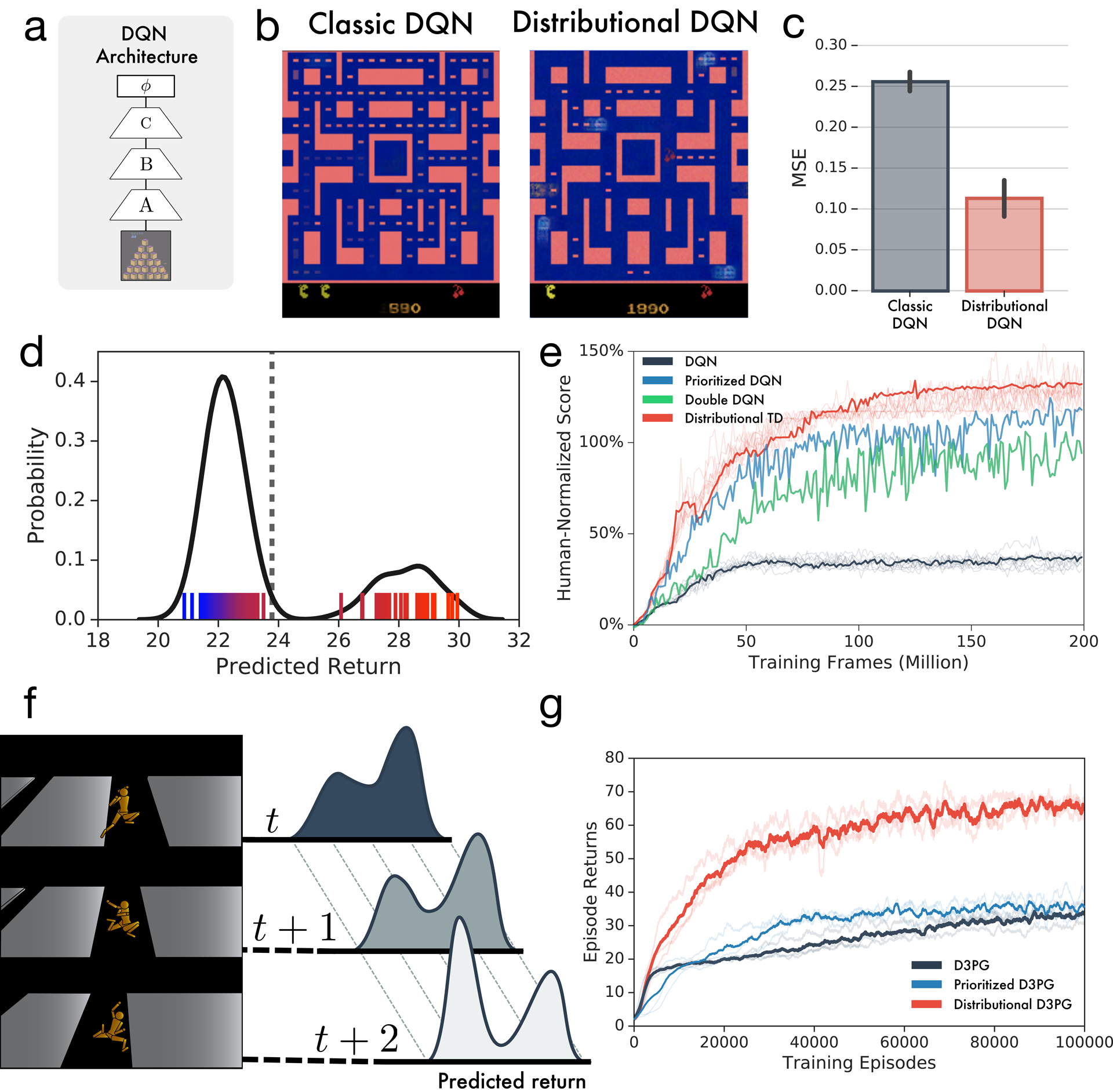
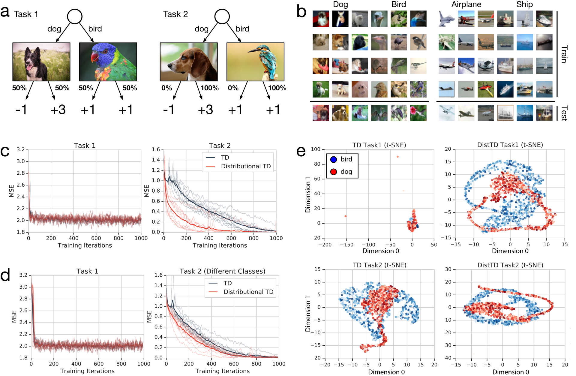
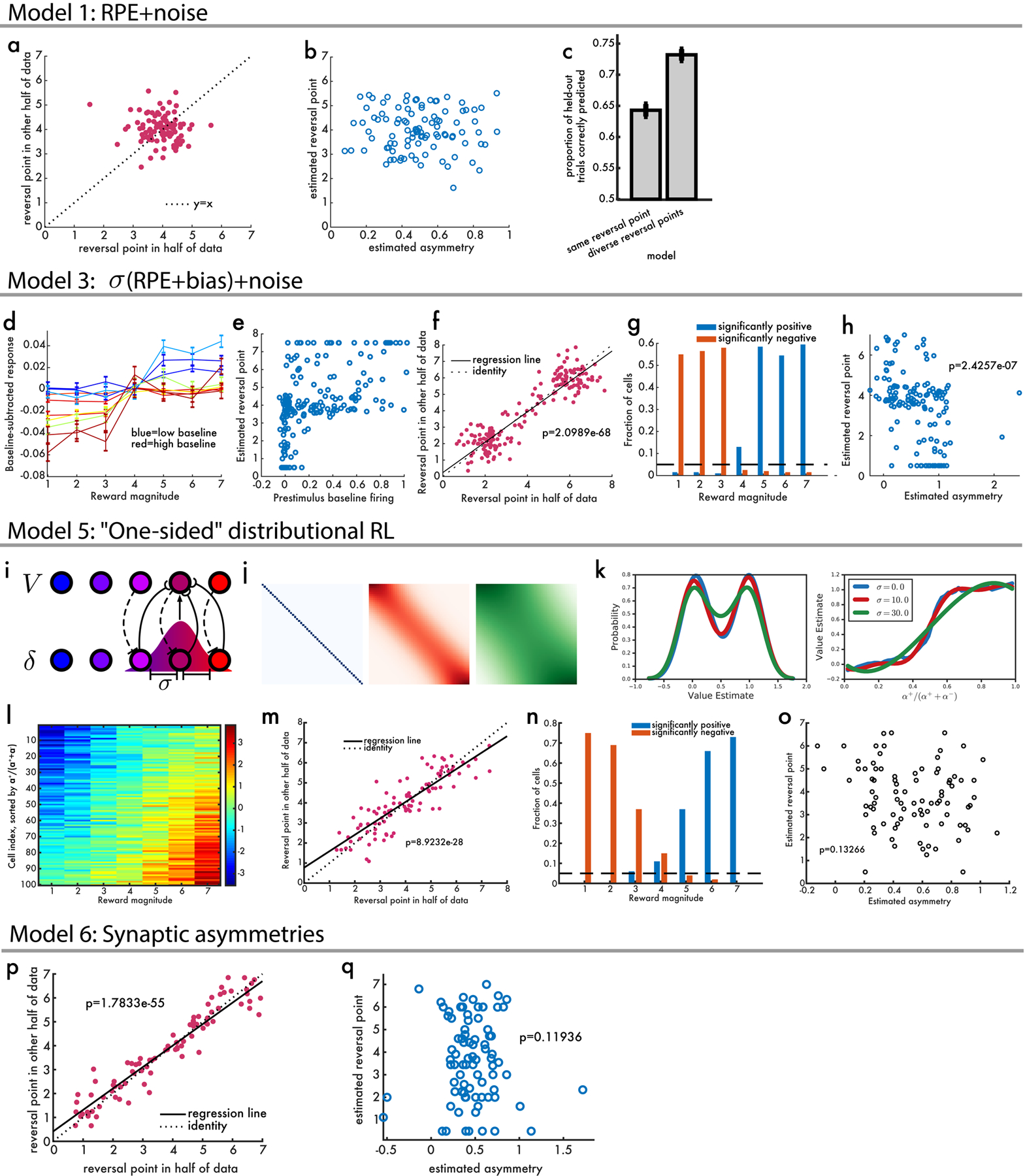
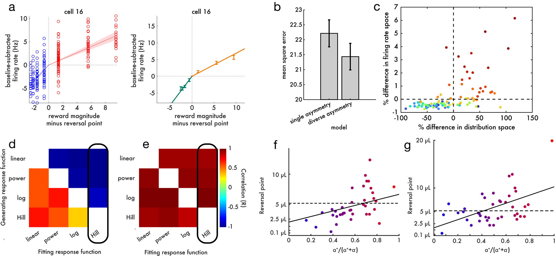
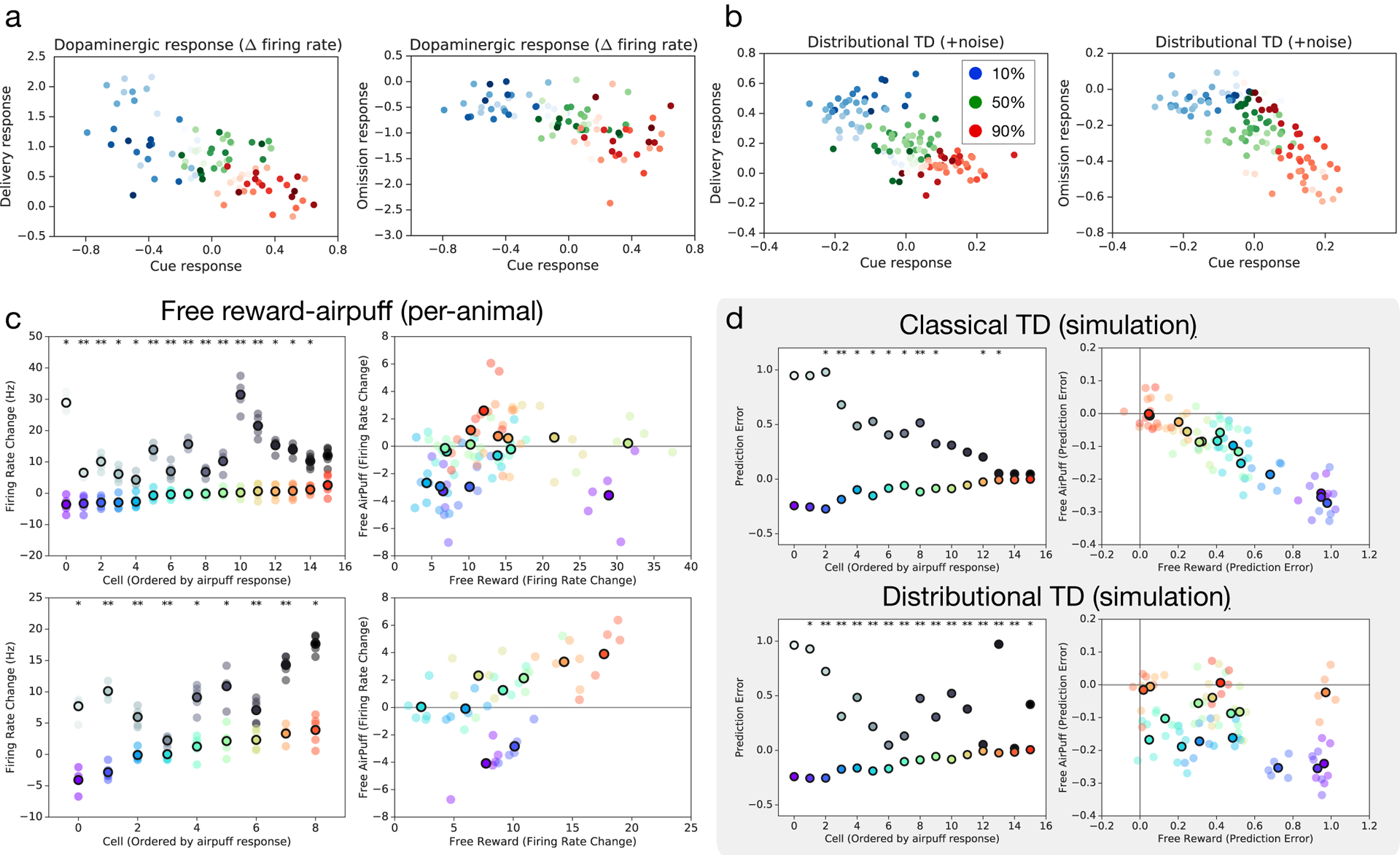
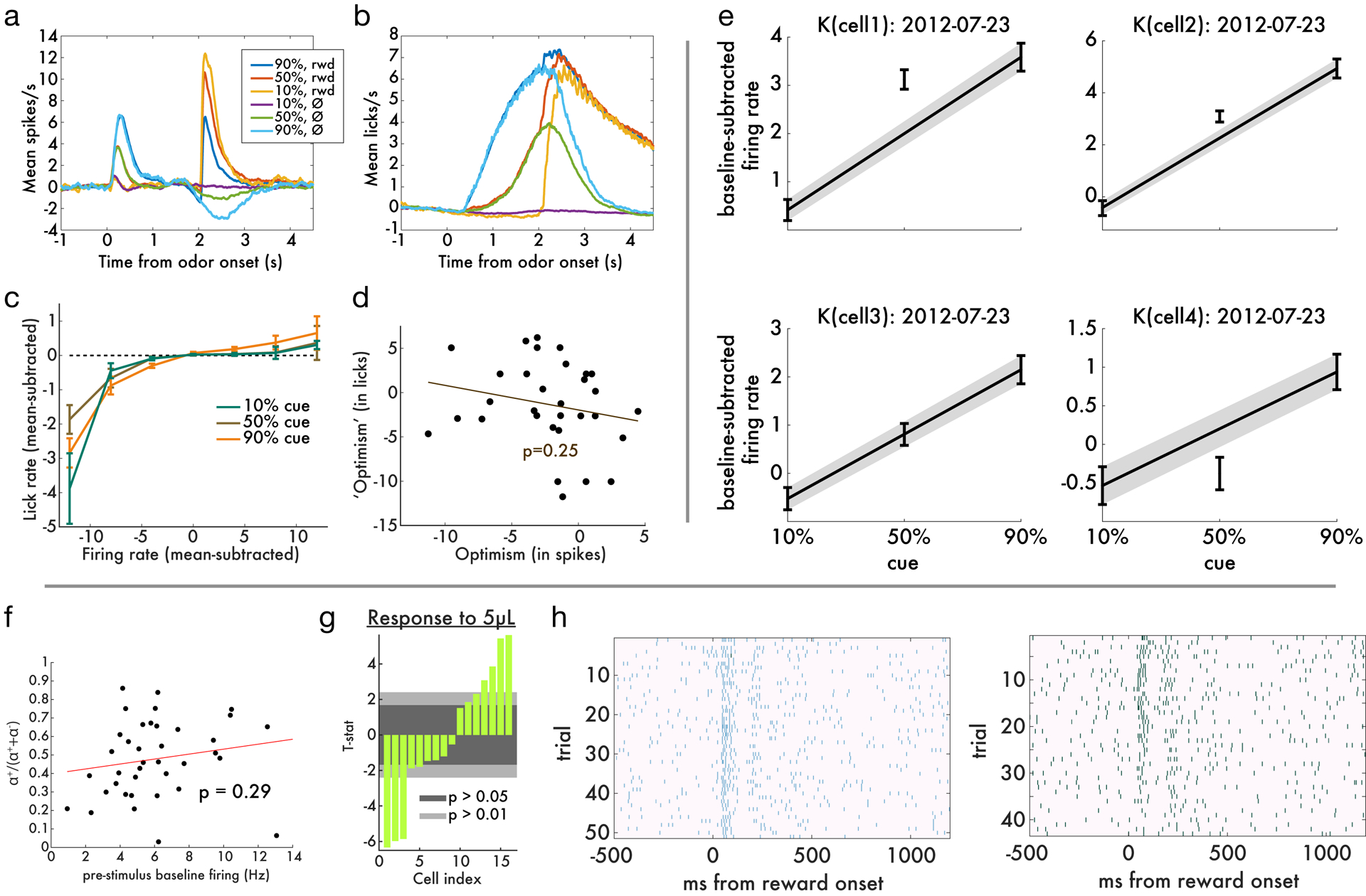
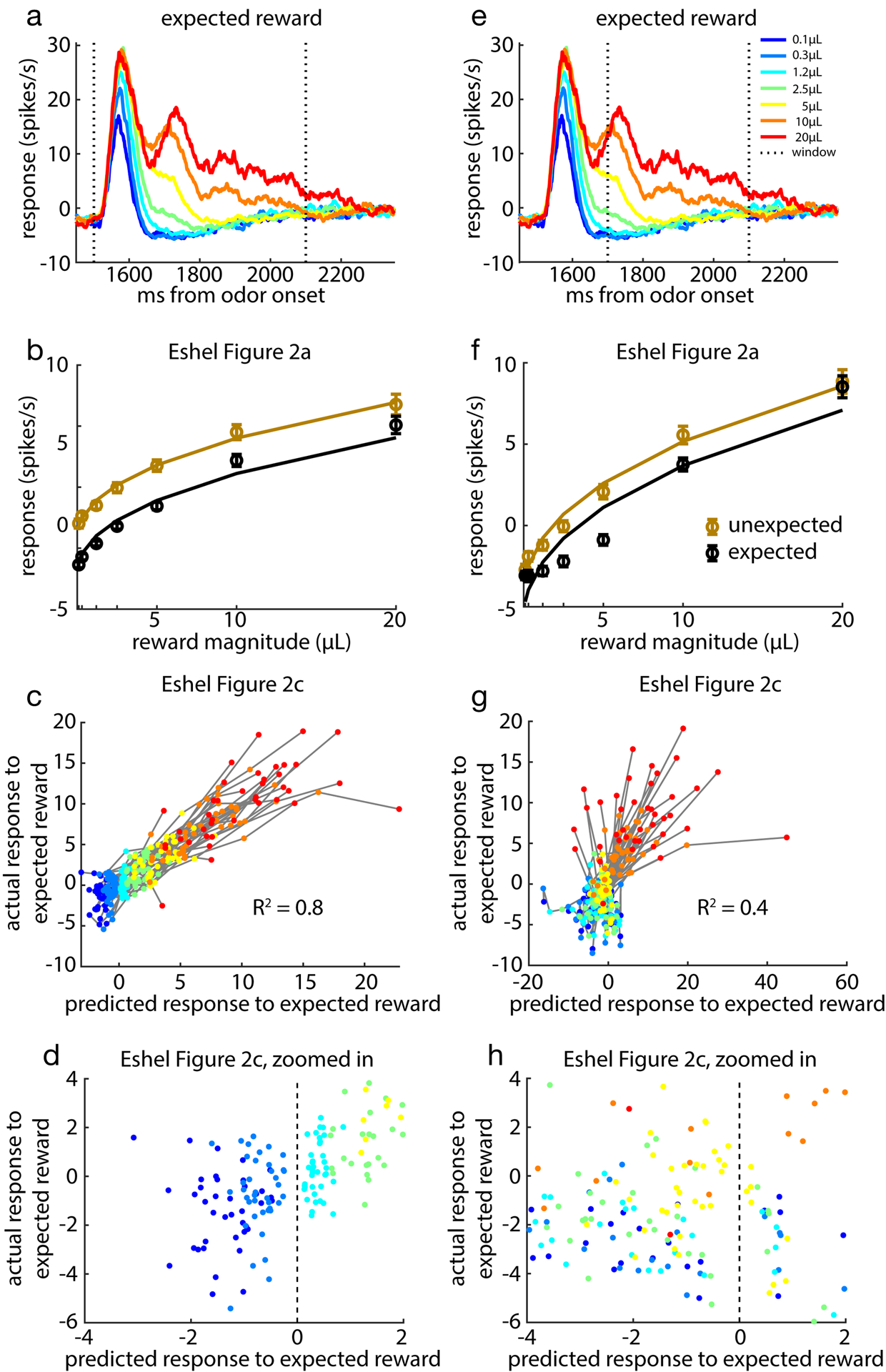
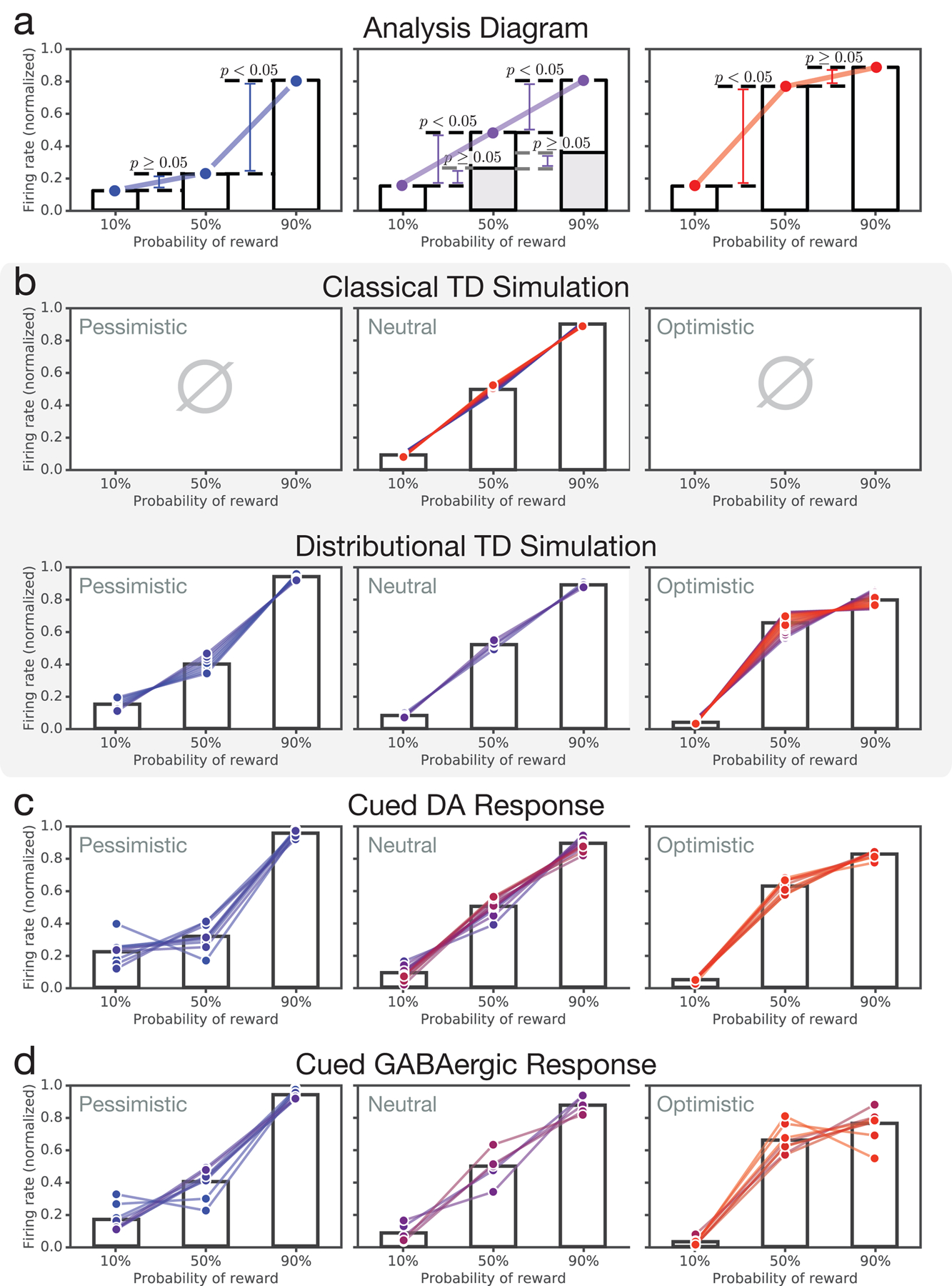
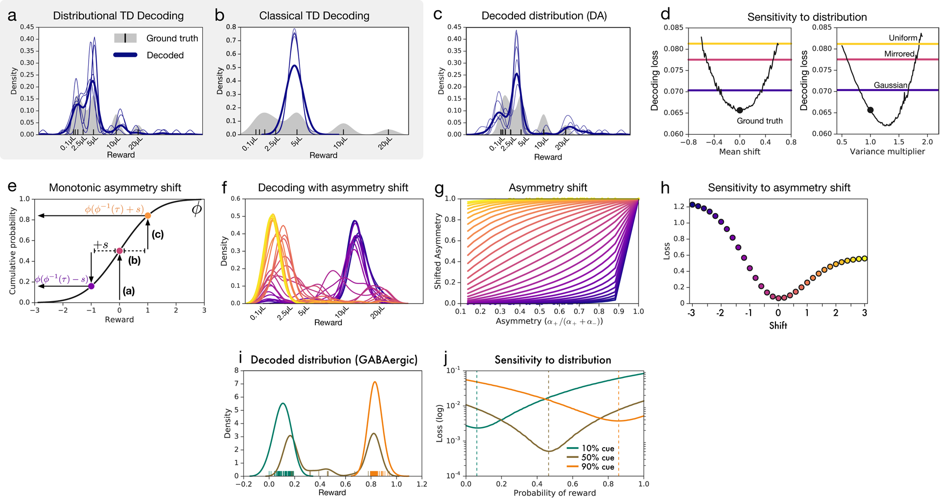
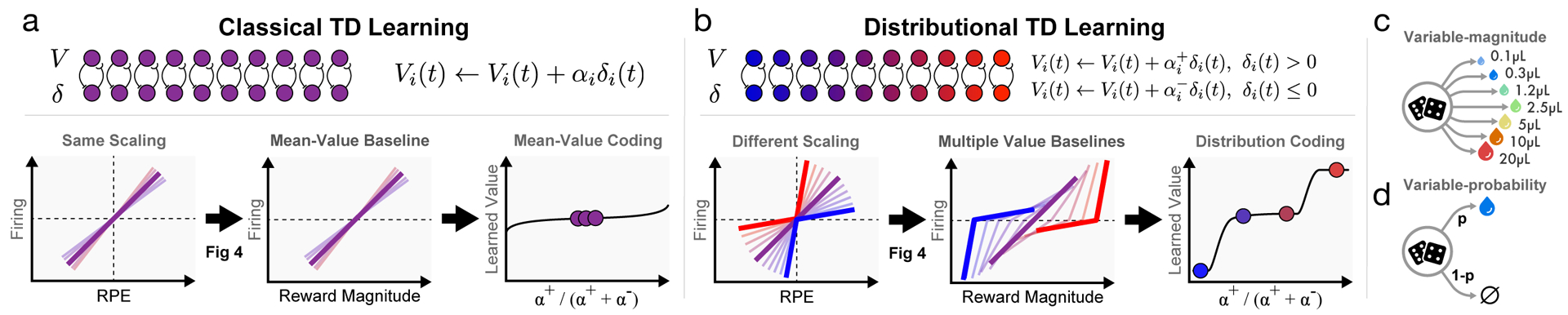
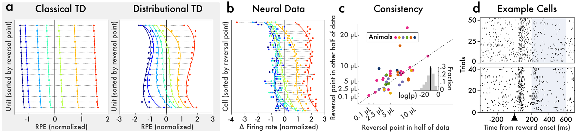
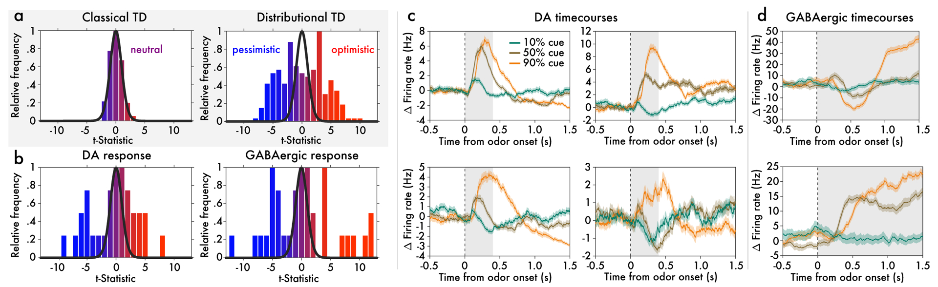
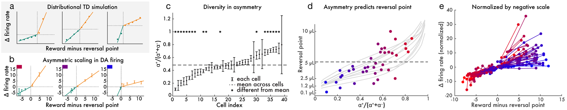
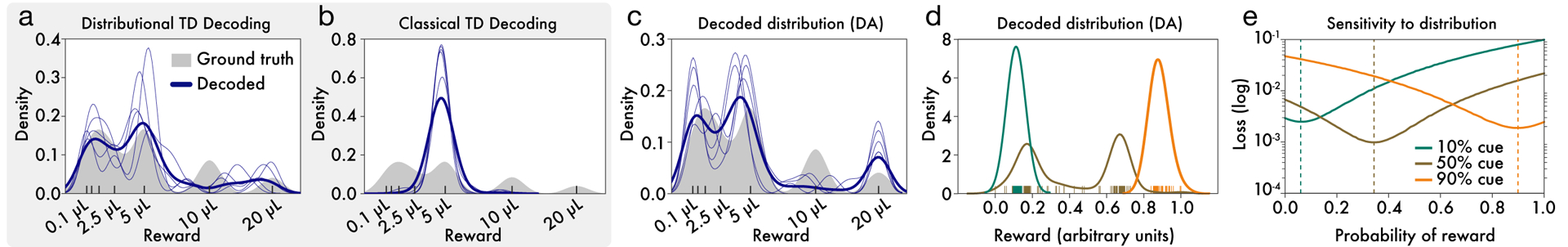
Since its introduction, the reward prediction error theory of dopamine has explained a wealth of empirical phenomena, providing a unifying framework for understanding the representation of reward and value in the brain^1-3. According to the now canonical theory, reward predictions are represented as a single scalar quantity, which supports learning about the expectation, or mean, of stochastic outcomes. Here we propose an account of dopamine-based reinforcement learning inspired by recent artificial intelligence research on distributional reinforcement learning^4-6. We hypothesized that the brain represents possible future rewards not as a single mean, but instead as a probability distribution, effectively representing multiple future outcomes simultaneously and in parallel. This idea implies a set of empirical predictions, which we tested using single-unit recordings from mouse ventral tegmental area. Our findings provide strong evidence for a neural realization of distributional reinforcement learning.

Extended Data Figure 1:. Mechanism of distributional TD.

a, The degree of asymmetry in positive to negative scale determines the equilibrium where positive and negative errors balance. Equal scaling equilibrates at the mean, whereas a larger positive (negative) scaling produces an equilibrium above (below) the mean. b, Distributional prediction emerges through experience. Quantile (sign function) version is displayed here for clarity. Model is trained on arbitrary task with trimodal reward distribution. c, Same as (b), viewed in terms of cumulative distribution (left) or learned value for each predictor (quantile function) (right).

Extended Data Figure 2:. Learning the distribution of returns improves performance of deep RL agents across multiple domains.

a, DQN and Distributional TD share identical non-linear network structures. b-c, After training classic or distributional DQN on MsPacman, we freeze the agent and then train a separate linear decoder to reconstruct frames from the agent’s final layer representation. For each agent, reconstructions are shown. The distributional model’s representation allows significantly better reconstruction. d, At a single frame of MsPacman (not shown), the agent’s value predictions together represent a probability distribution over future rewards. Reward predictions of individual RPE channels shown as tick marks ranging from pessimistic (blue) to optimistic (red), and kernel density estimate shown in black. e, Atari-57 experiments with single runs of prioritized experience replay and double DQN agents for reference. Benefits of distributional learning exceed other popular innovations. f-g, The performance payoff of distributional RL can be seen across a wide diversity of tasks. Here we give another example, a humanoid motor-control task in the MuJoCo physics simulator. Prioritized experience replay agent is shown for reference. Traces show individual runs, averages in bold.

Extended Data Figure 3:. Simulation experiment to examine the role of representation learning in distributional RL.

a, Illustration of tasks 1 and 2. b, Example images for each class used in our experiments. c, Experimental results, where each of 10 random seeds yields an individual run shown with traces, and bold gives average over seeds. d, Same as (c), but for control experiment. e, Bird-dog t-SNE visualization of final hidden layer of network, given different input images (bird=blue, dog=red). Left column shows classic TD and right column shows distributional TD. Top row shows the representation after training on task 1, and bottom row after training on task 2.

Extended Data Figure 4:. Null models.

a, Classical TD plus noise does not give rise to the pattern of results observed in real dopamine data in varible-magnitude task. When reversal points were estimated in two independent partitions there was no correlation between the two (p=0.32 by linear regression). b, We then estimated asymmetric scaling of responses and found no correlation between this and reversal point (p=0.78 by linear regression). c, Model comparison between ‘same’, a single reversal point, and ‘diverse’, separate reversal points. In both, the model is used to predict whether a held-out trial has a positive or negative response. d, Simulated baseline-subtracted RPEs, color-coded according to the ground-truth value of bias added to that each cell’s RPEs. e, Across all simulated cells, there was a strong positive relationship between prestimulus baseline firing and the estimated reversal point. f, Two independent measurements of the reversal point were strongly correlated. g, The proportion of simulated cells that have significantly positive (blue) or negative (red) responses showed no magnitudes with both positive and negative responses. h, In the simulation, there was a significant negative relationship between the estimated asymmetry of each cell and its estimated reversal point (opposite that observed in neural data). i, Diagram illustrating a Gaussian weighted topological mapping between RPEs and value predictors. j, Varying the standard deviation of this Gaussian modulates the degree of coupling. k, In a task with equal chance of a reward 1.0 or 0.0, distributional TD with different levels of coupling shows robustness to the degree of coupling. l, When there is no coupling, a distributional code is not learned, but asymmetric scaling can cause spurious detection of diverse reversal points. m, Even though every cell has the same reward prediction they appear to have different reversal points. n, With this model, some cells may have significantly positive responses, and others significantly negative responses, in response to the same reward. o, But this model is unable to explain a positive correlation between asymmetric scaling and reversal points. p, Simulation of “synaptic” distributional RL, where learning rates but not firing rates are asymmetrically scaled. This model predicts diversity in reversal points between dopamine neurons. q, But it predicts no correlation between asymmetric scaling of firing rates, and reversal point.

Extended Data Figure 5:. Asymmetry and reversal.

a, Left, All data points (trials) from an example cell. The solid lines are linear fits to the positive and negative domains, and the shaded areas show 95% confidence intervals calculated with Bayesian regression. Right, the same cell plotted in the format of main text Figure 4b. b, Cross-validated model comparison on the dopamine data favors allowing each cell to have its own asymmetric scaling (p = 1.4e – 11 by paired t-test). The standard error of the mean appears large relative to the p-value because the p-value is computed using a paired test. c, Although the difference between single-asymmetry and diverse-asymmetry models was small in firing rate space, such small differences correspond to large differences in decoded distribution space (more details in Supplement). Each point is a TD simulation; color indicates the degree of diversity in asymmetric scaling within that simulation. d, We were interested in whether an apparent correlation between reversal point and asymmetry could arise as an artifact, due to a mismatch between the shape of the actual dopamine response function and the function used to fit it. Here we simulate the variable-magnitude task using a TD model without a true correlation between asymmetric scaling and reversal point. We then apply the same analysis pipeline as in the main paper, to measure the correlation (color axis) between asymmetric scaling and reversal point. We repeat this procedure 20 times with different dopamine response functions in the simulation, and different functions used to fit the positive and negative domains of the simulated data. The functions are sorted in increasing order of concavity. An artifact can emerge if the response function used to fit the data is less concave than the response function used to generate the data. For example, when generating data with a Hill function but fitting with a linear function, a positive correlation can be spuriously measured. e, When simulating data from the distributional TD model, where a true correlation exists between asymmetric scaling and reversal point, it is always possible to detect this positive correlation, even if the fitting response function is more concave than the generating response function. The black rectangle highlights the function used to fit real neural data in panel c. f, In this panel we analyze the real dopamine cell data identically to main text Figure 4d, but using Hill functions instead of linear functions to fit the positive and negative domains. Because the correlation between asymmetric scaling and reversal point still appears under these adversarial conditions, we can be confident it is not driven by this artifact. g, Same as main text Figure 4d, but using linear response function and linear utility function (instead of empirical utility).

Extended Data Figure 6:. Cue responses versus outcome responses, and more evidence for diversity.

a, In variable-probability task: firing at cue, versus firing at reward (left) or omission (right). Color brightness denotes asymmetry. b, Same as (a), but showing RPEs from distributional TD simulation. c, Data from Eshel et al. also included unpredicted rewards and unpredicted airpuffs. Top two panels show responses for all the cells recorded in one animal and bottom two panels show responses for all the cells of another animal. In the left two panels, the x-axis is the baseline-subtracted response to free reward, and the y-axis is the baseline-subtracted response to airpuff. Dots with black outlines are per-cell means, and un-outlined dots are means of disjoint subsets of trials indicating consistency of asymmetry. The right two panels plot the same data in a different way, with cells sorted along the x-axis by response to airpuff. Response to reward is shown in grayscale dots. Asterisks indicate significant difference in firing rates from one or both neighboring cells. d, Simulations for distributional but not classical TD produce diversity in relative response.

Extended Data Figure 7:. More details of data in variable-probability task.

a, Details of analysis method. Of the four possible outcomes of the two Mann-Whitney tests (described in Methods), two outcomes correspond to interpolation (middle) and one each to the pessimistic (left) and optimistic (right) groups. b, Simulation results for the classical TD and distributional TD models. Y-axis shows the average firing rate change, normalized to mean zero and unit variance, in response to each of the three cues. Each curve is one cell. The cells are split into panels according to a statistical test for type of probability coding (see Methods for details). Color indicates the degree of optimism or pessimism. Distributional TD predicts simultaneous optimistic and pessimistic coding of probability whereas classical TD predicts all cells have the same coding. c, Same as b, but using data from real dopamine neurons. The pattern of results closely matches the predictions from the distributional TD model. d, Same as b, using data from putative VTA GABAergic interneurons.

Extended Data Figure 8:. Further distribution decoding analysis.

This figure pertains to the variable-magnitude experiment. a-c, In the decoding shown in the main text, we constrained the support of the distribution to the range of the rewards in the task. Here, we applied the decoding analysis without constraining the output values. We find similar results, although with increased variance. d, We compare the quality of the decoded distribution against several controls. The real decoding is shown as black dots. In colored lines are reference distributions (uniform and Gaussian with the same mean and variance as the ground truth; and the ground truth mirrored). Black traces shift or scale the ground truth distribution by varying amounts. e, Nonlinear functions used to shift asymmetries, to measure degradation of decoded distribution. The normal cumulative distribution function ϕ is used to transform asymmetry τ. This is shifted by some value s and transformed back through the normal quantile function ϕ⁻¹. Positive values s increase the value of τ and negative values decrease the value of τ. f, Decoded distributions under different shifts, s. g, Plot of shifted asymmetries for values of s used. h, Quantification of match between decoded and ground truth distribution, for each s. i-j, Same as main text Figure 5d–e, but for putative GABAergic cells rather than dopamine cells.

Extended Data Figure 9:. Simultaneous diversity.

Variable-probability task. Mean spiking (a) and licking (b) activity in response to each of the three cues (indicating 10%, 50% or 90% probability of reward) at time 0, and in response to the outcome (reward or no reward) at time 2000 ms. c, Trial-to-trial variations in lick rates were strongly correlated with trial-to-trial variations in dopamine firing rates. Each cell’s mean is subtracted from each axis, and the x-axis is binned for ease of visualization. d, Dopaminergic coding of the 50% cue relative to the 10% and 90% cues (as shown in panel b) was not correlated with the same measure computed on lick rates. Therefore, between-session differences in cue preference, measured by anticipatory licking, cannot explain between-cell differences in optimism. e, Four simultaneously recorded dopamine neurons. These are the same four cells whose timecourses are shown in Figure 3c in the main text. f, Variable-magnitude task. Across cells, there was no relationship between asymmetric scaling of positive versus negative prediction errors, and baseline firing rates (R=0.18, p=0.29). Each point is a cell. These data are from dopamine neurons at reward delivery time. g, t-statistics of response to 5 μL reward compared to baseline firing rate, for all 16 cells from animal ‘D’. Some cells respond significantly above baseline and others significantly below. Cells are sorted by t-statistic. h, Spike rasters showing all trials where the 5 μL reward was delivered. The two panels are two example cells from the same animal with rasters shown in Figure 2 of the main text.

Extended Data Figure 10:. Relationship of results to Eshel et al (2016).

Here we reproduce results for the variable-magnitude task from Eshel et al. with two different time windows. a, Change in firing rate in response to cued reward delivery averaged over all cells. b, Comparing hill-function fit and response averaged over all cells for expected (cued) and unexpected reward delivery. c, Correlation between response predicted by scaled common response function and actual response to expected reward delivery. d, Zooming in on (c) shows correlation driven primarily by larger reward magnitudes. e-h, Repeating the above analysis for a window of 200 – 600ms.

Figure 1:. Distributional value coding arises from a diversity of relative scaling of positive and negative prediction errors.

a, In the standard temporal difference (TD) theory of the dopamine system, all value predictors learn the same value V. Each dopamine cell is assumed to have the same relative scaling for positive and negative RPEs (left). This causes each value prediction (or value baseline) to be the mean of the outcome distribution (middle). Dotted lines indicate zero RPE or pre-stimulus firing. b, In our proposed model, distributional TD, different channels have different relative scaling for positive (α⁺) and negative (α⁻) RPEs. Red shading indicates α⁺ > α⁻, and blue shading indicates α⁻> α⁺. An imbalance between α⁺ and α⁻ causes each channel to learn a different value prediction. This set of value predictions collectively represents the distribution over possible rewards. c, We analyze data from two tasks. In the variable-magnitude task, there is a single cue, followed by a reward of unpredictable magnitude. d, In the variable-probability task, there are three cues, which each signal a different probability of reward, and the reward magnitude is fixed.

Figure 2:. Different dopamine neurons consistently reverse from positive to negative responses at different reward magnitudes.

Variable-magnitude task from Eshel et al.. On each trial, the animal experiences one of seven possible reward magnitudes (0.1, 0.3, 1.2, 2.5, 5, 10, or 20 μL), selected randomly. a, RPEs produced by classical and distributional TD simulations. Each horizontal bar is one simulated neuron. Each dot color corresponds to a particular reward magnitude. The x-axis is the cell’s response (change in firing rate) when reward is delivered. Cells are sorted by reversal point. In classic TD, all cells carried approximately the same RPE signal. Note that the slight differences between cells arose from Gaussian noise added to the simulation; the differences between cells in the classic TD simulation were not statistically reliable. Conversely, in distributional TD, cells had reliably different degrees of optimism. Some responded positively to almost all rewards, and others responded positively to only the very largest reward. b, Responses recorded from light-identified dopamine neurons in behaving mice. Neurons differed markedly in their reversal points. c, To assess whether this diversity was reliable, we randomly partitioned the data into two halves and estimated reversal points independently in each half. We found that the reversal point estimated in one half was highly correlated with that estimated in the other half. d, Spike rasters for two example dopamine neurons from the same animal, showing responses to all trials when the 5 μL reward was delivered. We analyzed data from 200 to 600 ms after reward onset (highlighted), to exclude the initial transient which was positive for all magnitudes. During this epoch, the cell on the bottom fires above its baseline rate, while the cell on the top pauses.

Figure 3:. Optimistic and pessimistic probability coding occur concurrently in dopamine and VTA GABA neurons.

Data from variable-probability task. a, Histogram (across simulated cells) of t-statistics which compare each cell’s 50% cue response against the mean 50% cue response across cells. (Qualitatively identical results hold when comparing 50% cue response against midpoint of 10% and 90% responses.) The superimposed black curve shows the t-distribution with the corresponding degrees of freedom. Distributional TD predicts simultaneous optimistic and pessimistic coding of probability whereas classical TD predicts all cells have the same coding. Color indicates the degree of optimism or pessimism. b, Same as (a), but using data from real dopamine and putative GABA neurons. The pattern of results closely matches the predictions from the distributional TD model. c, Responses of four example dopamine neurons recorded simultaneously in a single animal. Each trace is the average response to one of the three cues. Time zero is the onset of the odor cue. Some cells code the 50% cue similarly to the 90% cue, while others simultaneously code it similarly to the 10% cue. Gray areas show epoch averaged for summary analyses. d, Responses of two example VTA GABAergic cells from the same animal.

Figure 4:. Relative scaling of positive and negative dopamine responses predicts reversal point.

a, Three simulated dopamine neurons – each with a different asymmetry – in the variable-magnitude task. For each unit, we empirically estimated the reversal point where responses switch from negative to positive. The x-axis shows reward minus the per-cell reversal point, effectively aligning each cell’s responses to its respective reversal point. Baseline-subtracted response to reward is plotted on y-axis. Responses below the reversal point are shown in green and those above are shown in orange. Solid curves show linear functions fit separately to the above-reversal and below-reversal domains of each cell. b, Same as (a), but showing three real example dopamine cells. c, The diversity in relative scaling of positive and negative responses in dopamine cells is statistically reliable. The 95% confidence intervals of α⁺/(α⁺ + α⁻) are displayed, where α⁺ and α⁻ are the slopes estimated above. d, Relative scaling of positive and negative responses predicts that cell’s reversal point (each point is one dopamine cell). Dashed line is the mean over cells. Light gray traces show reversal points measured in distributional TD simulations of the same task, and show variability over simulation runs. e, All 40 dopamine cells plotted in the same fashion as in b, except normalized by the slope estimated in the negative domain. Thus, the observed variability in slope in the positive domain corresponds to diversity in relative scaling of positive and negative responses. Cells are colored by reversal point, to illustrate the relationship between reversal point and asymmetric scaling. In all panels, reward magnitudes are in estimated utility space (see Methods).

Figure 5:. Decoding reward distributions from neural responses.

a, Distributional TD simulation trained on the variable-magnitude task, whose actual (smoothed) distribution of rewards is shown in gray. After training the model, we interpret the learned values as a set of expectiles. We then decode the set of expectiles into a probability density (blue traces). Multiple solutions are shown in light blue, and the average across solutions is shown in dark blue. (See Methods for more details.) b, Same as(a), but with a classical TD simulation. c, Same as (a), but using data from recorded dopamine cells. The expectiles are defined by the reversal points and the relative scaling from the slopes of positive and negative RPEs, as shown in Figure 5. Unlike the classic TD simulation, the real dopamine cells collectively encode the shape of the reward distribution that animals have been trained to expect. d Same decoding analysis, using data from each of the cue conditions in the variable-probability task, based on cue responses of dopamine neurons (decoding for GABA neurons shown in Extended Data Figure 8 i,j). e, The neural data for both dopamine and GABA neurons were best fit by Bernoulli distributions closely approximating the ground-truth reward probabilities in all three cue conditions.

References

1. Schultz Wolfram, Wiliam R Stauffer, and Armin Lak. The phasic dopamine signal maturing: from reward via behavioural activation to formal economic utility. Current opinion in neurobiology, 43: 139–148, 2017. - PubMed
1. Glimcher Paul W. Understanding dopamine and reinforcement learning: the dopamine reward prediction error hypothesis. Proceedings of the National Academy of Sciences, 108(Supplement 3):15647–15654, 2011. - PMC - PubMed
1. Watabe-Uchida Mitsuko, Eshel Neir, and Uchida Naoshige. Neural circuitry of reward prediction error. Annual review of neuroscience, 40:373–394, 2017. - PMC - PubMed
1. Morimura Tetsuro, Sugiyama Masashi, Kashima Hisashi, Hachiya Hirotaka, and Tanaka Toshiyuki. Parametric return density estimation for reinforcement learning In Proceedings of the Twenty-Sixth Conference on Uncertainty in Artificial Intelligence, UAI’10, pages 368–375, Arlington, Virginia, United States, 2010. AUAI Press; ISBN 978-0-9749039-6-5. URL http://dl.acm.org/citation.cfm?id=3023549.3023592.
1. Marc G Bellemare Will Dabney, and Munos Rémi. A distributional perspective on reinforcement learning. In International Conference on Machine Learning, pages 449–458, 2017.