Cellular Dialogues: Cell-Cell Communication through Diffusible Molecules Yields Dynamic Spatial Patterns

Abstract

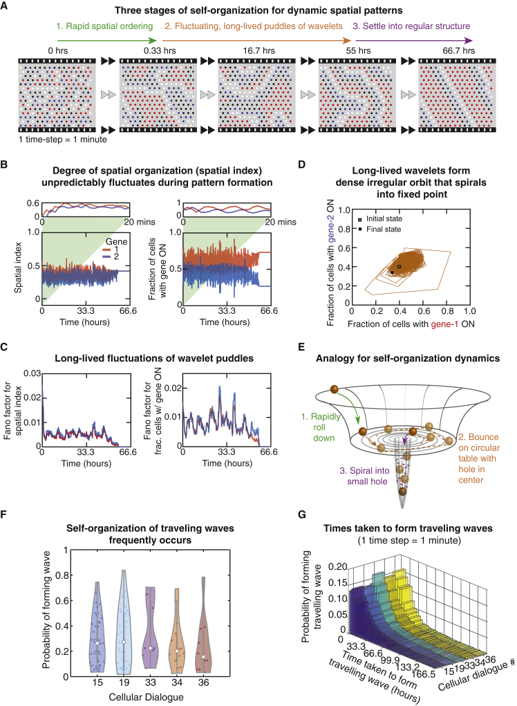
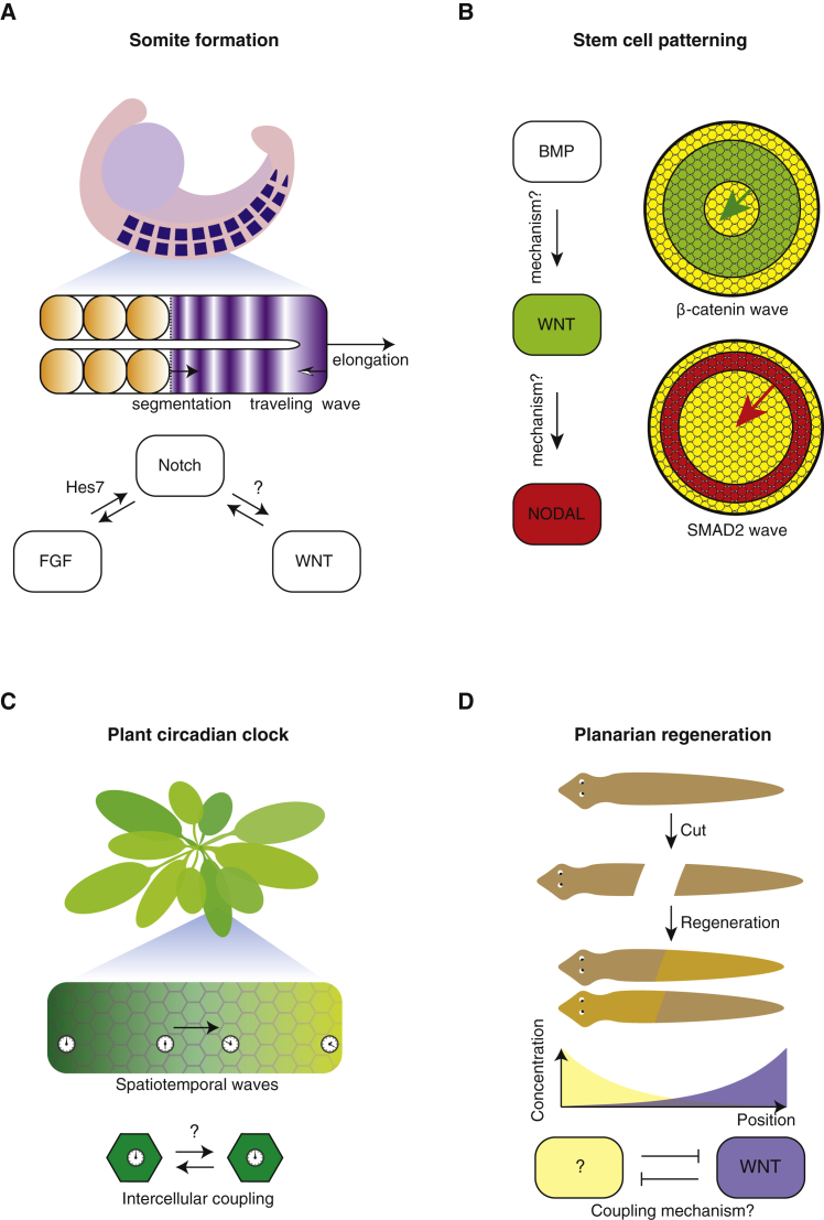
Cells form spatial patterns by coordinating their gene expressions. How a group of mesoscopic numbers (hundreds to thousands) of cells, without pre-existing morphogen gradients and spatial organization, self-organizes spatial patterns remains poorly understood. Of particular importance are dynamic spatial patterns such as spiral waves that perpetually move and transmit information. We developed an open-source software for simulating a field of cells that communicate by secreting any number of molecules. With this software and a theory, we identified all possible "cellular dialogues"-ways of communicating with two diffusing molecules-that yield diverse dynamic spatial patterns. These patterns emerge despite widely varying responses of cells to the molecules, gene-expression noise, spatial arrangements, and cell movements. A three-stage, "order-fluctuate-settle" process forms dynamic spatial patterns: cells form long-lived whirlpools of wavelets that, following erratic dynamics, settle into a dynamic spatial pattern. Our work helps in identifying gene-regulatory networks that underlie dynamic pattern formations.

Keywords: cell-cell communication; cellular automata; complex systems; gene networks; multicellular systems; pattern formation; reaction-diffusion; self organization; spatial patterns; waves.

Graphical abstract

Figure 1

Computationally Screening Cellular Dialogues to Find Ones that Enable Dynamic Patterns to Form (A) Pattern formation by cells versus chemicals. (Top) Mechanisms by which an initially disordered field of a mesoscopic number of cells (∼hundreds to thousands) (left panel) become more ordered through cell-cell communication (right panel) remain poorly understood, as is the method to analyze this complex self-organization dynamics. (Bottom) A field of chemicals or a continuum of cells (large number of tightly packed cells) initially having no pattern (left) can form a pattern (right) without pre-existing morphogens. This is usually modeled by reaction-diffusion equations and can be understood through the Turing mechanism. (B) Static versus dynamic patterns. (Top) Static patterns do not change over time. (Bottom) In dynamic patterns, a structure changes over time without ever stopping (e.g., shown here is a traveling wave). (C) Schematic of cellular dialogues. Brown (molecule-1) and green (molecule-2) circles are ligands that bind to their cognate receptors on the cell membrane. Ligand-bound receptors trigger intracellular signal transductions that either positively or negatively regulate the production and secretion of molecules-1 and 2 (molecule-1 can self-promote or self-repress its own secretion while also regulating the secretion of molecule-2, and vice versa). Bottom row shows graphic representation of cellular dialogues. (D) Elements that we varied in simulations: cellular dialogues of all possible topologies, the values of the parameters for each cellular dialogue, and spatial arrangement of cells. Our study first begins with an infinite Hill coefficient (i.e., digital response to each of the two signaling molecules) and a regular lattice. After reporting the outcomes of these simulations, we report the result of relaxing these two constraints and well as other elements not depicted. See also Figure S1.

Figure 2

Examples of Self-Organized Dynamic Patterns Found through Computational Screening In all the figures shown here, a cell (drawn as a circle) can have four colors. Each color represents a distinct gene expression state, (gene 1 = ON/OFF, gene 2 = ON/OFF): black means (ON, ON), red means (ON, OFF), blue means (OFF, ON), and white means (OFF, OFF). In all the simulations, a field of cells starts with a completely spatial disordered configuration—there is no correlation between neighboring cells' gene expression states—as exemplified by the leftmost picture shown in (A). (A) Traveling wave of horizontal bands. Snapshots of the formation process shown at different stages of a simulation. Assuming that one time step in the simulation takes one min, the clocks show time passed from noon (beginning of the simulation). (B) Complex pool of multiple wavelets formed, starting with a spatially disorganized field of cells. Snapshots at different stages of the simulation are shown. Assuming that one time step represents 1 min, the clock and the days elapsed indicate at which time steps in the simulation the snapshots are taken. (C–J) Each filmstrip shows three non-contiguous snapshots of a moving, dynamic pattern that formed, starting from a spatially disorganized configuration (not shown, see examples in the first snapshots in (A). Where shown, the arrows represent the direction of travel. The dynamic patterns are: (C) a single traveling horizontal band, (D) traveling vertical bands, (E) a traveling zigzag band, (F) a spiral wave, (G) traveling diagonal bands, (H) a small island of cells (enclosed in the blue hexagon) oscillating over time while all cells outside the island remain static, (I) every cell oscillates between red and blue with period 2, and (J) seemingly erratic, never-ending dynamics in which multiple wavelets form and meet and annihilate each other with the pool of wavelets constantly evolving and never repeating the same configuration throughout the simulation.

Figure 3

Computational Search Revealed Tree Structures that Group Cellular Dialogues Based on Their Ability to Generate Either Static Patterns, Dynamic Temporal Patterns, or Dynamic Spatial Patterns (A) Two classes of dynamic patterns. (Top) Dynamic temporal patterns repeat themselves over time without transmitting information across space. (Bottom) Dynamic spatial patterns involve cells that transmit information over space through a coherent structure that moves across the field. (B–D) Tree diagrams show a full classification of all 44 unique, non-trivial cellular dialogues into three distinct classes (see STAR Methods). In each tree diagram, a cellular dialogue is a leaf (box) that is joined by branches to other cellular dialogues. As one moves from one leaf to the next, an edge is either removed or added to the cellular dialogue. (B) Tree diagram showing all cellular dialogues that cannot generate any dynamic patterns. All cellular dialogues here lack mutual interactions and self-repressions. (C) Tree diagram showing all cellular dialogues that can generate dynamic temporal patterns but not dynamic spatial patterns. These all have either a self-repression (red boxes), a mutual interaction of the same sign (blue boxes), or both (purple boxes). Cellular dialogue 14 is an exception—it has mutual interactions of different signs and no self-interactions. (D) Tree diagram showing all cellular dialogues that can generate dynamic spatial patterns, as well as dynamic temporal patterns. These are all generated by adding at least one additional self-interaction to cellular dialogue 14. Cellular dialogues in the five red boxes have at least one positive feedback loop and can generate non-oscillatory dynamic spatial patterns (e.g., traveling waves). Cellular dialogues in the blue boxes have only negative self-interactions and produce dynamic spatial patterns but always with a concurrent dynamic temporal pattern (e.g., a traveling wave where the cells oscillate simultaneously) (see Figure S3 for examples). (E) The maximum observed simulation time is a metric that naturally separates the three classes of cellular dialogues (B–D) (see Figure S4 for other metrics). A node represents a cellular dialogue and the node's shape represents the type of cellular dialogue (one of the three B–D). A node's color indicates the longest observed simulation time among a large set of simulations that were performed with different parameters. See also Figures S2–S4.

Figure 4

Analytic Framework Predicts and Explains How Cells Can Sustain Dynamic Spatial Patterns (A–C) Three-step overview of an analytic (pen and paper) approach to understanding the simulations (see Supplemental Analysis Section S3 for details). (A) Step 1: decompose straight (top) and bent (bottom) waves into distinct layers of cells. Cells of the same layer have the same gene expression state. (B) Step 2: estimate the total concentrations of molecules that a cell senses by exactly calculating the portions of those concentrations that are due to the cell itself and its nearest neighbors and by approximating the portions of the total concentrations that are due to further-away cells. (C) Step 3: (right) Directed graph-representation showing how a cell must transition to distinct layers shown in (A) at each time step, which is explained by six mathematical inequalities that are derived through step 2. (D) Numerically solving the six inequalities in (C) shows that only two types of waves, shown here are possible and which cellular dialogues can produce them (cellular dialogues 15, 36, and 33 for wave type 1; cellular dialogues 19, 33, and 34 for wave type 2). (E) Adding self-activation to cellular dialogue 14 yields, in the left column, cellular dialogues 15 and 19. Directed graph -representation showing the gene expression transitions of a cell for each cellular dialogue (see Supplemental Analysis Section S2). (F) Parameter values that allow for sustaining of rectilinear waves, when represented as red points, form a dense region (red region) as shown in these spider charts. These parameter values satisfy the six inequalities derived by the analytic theory (C) (see Figure S6C for a direct comparison with parameter values found purely through computational search). The spider charts show the following parameters: threshold concentrations $K^{\left(ij\right)}$ for each molecular interaction and the maximum secretion rate $C_{ON}^{\left(j\right)}$ for each of the two molecules. See also Figures S5 and S6.

Figure 5

Three-Step, “Order-Fluctuate-Settle” Process Leads to Formation of Dynamic Spatial Patterns (A) Snapshots of a simulation showing the three stages of a traveling-wave formation—the three stages are described above the filmstrip. Assuming that one time step of a simulation represents 1 min, indicated above each snapshot is the elapsed time in hours. Color scheme for cells is the same as in Figure 2. (B) Two macroscopic parameters—the spatial index and the fractions of cells with a particular gene ON—plotted as a function of time for the wave-forming simulation shown in (A). 1 min represents one timestep. (Left panel) the spatial index—with magnitude between zero and one—measures the degree of spatial organization (zero means complete disorder, i.e., no spatial correlation in gene expression among cells and increasing values correspond to more spatial organization). Inset shows the spatial index rapidly increasing for the first twenty time steps. Spatial index for gene 1 (red) and gene 2 (blue). (Right panel) Fractions of cells with gene 1 ON (red) and of gene 2 ON (blue) for a typical wave-formation process. Inset shows the first twenty time steps. (C) For data in (B) and genes 1 (red) and 2 (blue), we used a moving window to compute the moving coefficient of variations in the spatial index (left panel) and in the fractions of cells with the specified gene ON (see STAR Methods). (D) For a typical simulation that self-organizes into a traveling wave, we plot the trajectory in phase space formed by the fractions of cells with gene 1 ON and gene 2 ON. The trajectory begins at the square (first time step of the simulation) and terminates at the circle (last time step of the simulation). (E) Analogy for the three-stage self-organization process—a billiard ball rolls down a bowl, bounces around on the flat circular bottom, and then fall through a tunnel after finding a small hole drilled into the circular bottom. (F) Probability of forming a traveling wave for each of the five cellular dialogues (detailed results in Figure S8). Violin plots showing the non-parametric kernel density (colored distributions), together with the median (white circle), interquartile range (thick vertical line) and 1.5× interquartile range (thin vertical line). Results are obtained by running 500 simulations for each of the parameter sets for which at least one traveling wave formed in the computational screening (see STAR Methods). Individual dots represent probabilities for individual parameter sets. (G) Distributions of the time taken to form traveling waves for each of the five cellular dialogues that enable cells to form dynamic spatial patterns (detailed results in Figure S10). See also Figures S7–S10.

Figure 6

Dynamic Spatial Patterns Still Form Even with More Complex Elements (A) Schematic of four additional, more complex elements that we added to our computational screen. (B) We examined two features with the elements in (A): (Top) can a disorganized field of cells still self-organize dynamic spatial patterns? (Bottom) Starting with a traveling wave, can the cells sustain it? (C) Examples of dynamic spatial patterns formed for each of the elements shown in (A). Colored boxes that enclose the filmstrips correspond to the colors used for each element shown in (A). (D) Fraction of simulations that form a dynamic pattern as a function of the deviation from the more idealized setting—cells placed on a regular lattice and responding digitally with an infinite Hill coefficient—in which the results for Figures 1, 2, 3, 4, and 5 were reported. Four colored boxes with each color corresponding to colored box in (A) that shows the modified element in the simulations. For each data point, we ran a large set of simulations with a fixed set of initial conditions as we varied the parameter controlling the deviation from our original model and classified their final states (see Figure S11 for details on finite Hill coefficient and noise). All results here are for cellular dialogue 15. (E) Fraction of simulations with cellular dialogue 15 that can sustain a traveling wave for at least one full period after starting with a traveling wave. We took parameter values for which the simulations with simpler elements (i.e., infinite Hill coefficient and cells on a regular lattice) can propagate traveling waves. See also Figures S11–S14.

Figure 7

Self-Organized Dynamic-Pattern-Forming Systems with Poorly Understood Interactions that Our Software and Analytic Framework May Help in Elucidating (A–D) Biological systems with two or more interacting pathways that generate spatiotemporal patterns but whose exact mechanisms and cellular dialogues remain poorly understood. (A) During somitogenesis, a wave of gene expression states propagates along the anterior-posterior axis of an elongating, pre-somite mesoderm. The conventional view is that this wave is mediated by a coupling between individual oscillators—oscillations in expression levels of Wnt, Notch, and Fgf and/or by large-scale gradients in the gene expression levels for those molecules. But how Notch regulates Wnt and vice versa remains questionable while Hes7 is known to mediate the Fgf-Notch interaction (Sonnen et al., 2018). Figure partially adapted from (Oates et al., 2012). (B) Waves of β-catenin (green ring) and Smad2 (red ring) expression levels propagate in a field of stem cells. Although we know that these waves form because of BMP inducing β-catenin (part of the Wnt pathway) and SMAD2 (part of the NODAL pathway), how exactly these two inductions occur remains poorly understood (Chhabra et al., 2019). (C) The circadian clocks of each cell within the leaf of Arabidoposis thaliana are thought to be coupled to each other through an as-yet-unknown mechanism, which is suspected to involve a variety of hormones, sugars, mRNAs, and other molecules (Greenwood et al., 2019). (D) A planarian regenerates itself after being cut into two or more pieces. This is thought to rely on mutual antagonism between gradients of Wnt expression (purple) and of an as-yet-unidentified molecule (yellow) (Stückemann et al., 2017). Figure partially adapted from (Stückemann et al., 2017).

References

1. Alon U. First edition. CRC Press; 2006. An introduction to systems biology: design principles of biological circuits.
1. Bar-Yam Y. First edition. Avalon Publishing; 2003. Dynamics of complex systems.
1. Buchler N.E., Gerland U., Hwa T. On schemes of combinatorial transcription logic. Proc. Natl. Acad. Sci. USA. 2003;100:5136–5141. - PMC - PubMed
1. Chen C.C., Wang L., Plikus M.V., Jiang T.X., Murray P.J., Ramos R., Guerrero-Juarez C.F., Hughes M.W., Lee O.K., Shi S. Organ-level quorum sensing directs regeneration in hair stem cell populations. Cell. 2015;161:277–290. - PMC - PubMed
1. Chhabra S., Liu L., Goh R., Kong X., Warmflash A. Dissecting the dynamics of signaling events in the BMP, WNT, and NODAL cascade during self-organized fate patterning in human gastruloids. PLoS Biol. 2019;17:e3000498. - PMC - PubMed
Publication types
LinkOut - more resources