Optimal memory-aware backpropagation of deep join networks

Abstract

Deep learning training memory needs can prevent the user from considering large models and large batch sizes. In this work, we propose to use techniques from memory-aware scheduling and automatic differentiation (AD) to execute a backpropagation graph with a bounded memory requirement at the cost of extra recomputations. The case of a single homogeneous chain, i.e. the case of a network whose stages are all identical and form a chain, is well understood and optimal solutions have been proposed in the AD literature. The networks encountered in practice in the context of deep learning are much more diverse, both in terms of shape and heterogeneity. In this work, we define the class of backpropagation graphs, and extend those on which one can compute in polynomial time a solution that minimizes the total number of recomputations. In particular, we consider join graphs which correspond to models such as siamese or cross-modal networks. This article is part of a discussion meeting issue 'Numerical algorithms for high-performance computational science'.

Keywords: backpropagation; memory; pebble game.

Figure 1.

Data dependencies of the backpropagation graph corresponding to the transformation of a linear chain. Functions are modelled by grey vertices, arrows represent data dependencies (input/output of functions) where the data are either x_i and ${\overline{x}}_i$. The chain is the graph on top, its dual graph is on the bottom.

Figure 2.

A join graph with three branches of respective length 5, 4 and 6.

Figure 3.

Data dependencies in the multiple adjoint chains problem with two chains. In the following, we call forward (resp. backward) data the output of F (resp. $\overline{F}$) functions.

Figure 4.

The three main phases of the algorithm. Green blocks correspond to the storage of ‘forward’ data, blue blocks to storage of ‘backward’ data. To process the backward phase, the red-circled value stored during the forward phase is used to recompute subsequent values. (a) The forward phase, (b) the turn, (c) the backward phase. (Online version in colour.)

Figure 5.

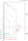
A canonical solution on the join with three branches of respective lengths 4 (blue), 10 (green) and 12 (red), with nine memory slots. The execution time is represented on the vertical axis, the progress on each of the branches is represented on the horizontal axis. As an example, the dark dashed line at the top of the figure represent the computation of $F_2^{(3)}$. Full (resp. dashed) vertical lines are memory checkpoints of forward data (resp. backward data). $\mathrm{Rev}(l,c)$ is the solution [10] to the easier problem where there is only one branch of size l and c checkpoints (figure 1), Opt₀ (l, c) is its execution time. (Online version in colour.)

Figure 6.

The three key properties of a canonical solution. Green blocks correspond to ‘forward’ data being stored, blue blocks to ‘backward’ data stored. The forbidden operations given by the properties are crossed out in red. For Stability 2, if during the backward phase, we have read the circled checkpoint, then the canonical solution starts by backpropagating (represented by the back arrow) all greyed-out operations until the ‘backward’ data of the circled-out operation is stored. (a) Stability 1, (b) checkpoint persistence, (c) Stability 2. (Online version in colour.)

Figure 7.

Makespan evolution with respect to different amount of total memory. (a) L = 5, (b) L = 15. (Online version in colour.)

Figure 8.

Makespan evolution with respect to different L for fixed memory size c. (a) c = 9, (b) c = 13. (Online version in colour.)

Figure 9.

Graph transformation (a) and performance (b). (a) Transformation of a join with three branches into a chain with four levels, (b) performance of Equiv-Chain versus Optimal. (Online version in colour.)

References

1. Glorot X, Bengio Y. 2010. Understanding the difficulty of training deep feedforward neural networks. In Proc. of the thirteenth Int. Conf. on Artificial Intelligence and Statistics, pp. 249–256.
1. Dean J.et al.2012Large scale distributed deep networks. In Advances in neural information processing systems, pp. 1223–1231. (https://papers.nips.cc/paper/4687-large-scale-distributed-deep-networks)
1. Das D, Avancha S, Mudigere D, Vaidynathan K, Sridharan S, Kalamkar D, Kaul B, Dubey P. 2016 Distributed deep learning using synchronous stochastic gradient descent. (http://arxiv.org/abs/1602.06709. )
1. Sethi R. 1975. Complete register allocation problems. SIAM J. Comput. 4, 226–248. (10.1137/0204020) - DOI
1. Liu JWH. 1987. An application of generalized tree pebbling to sparse matrix factorization. SIAM J. Algebr. Discret. Methods 8, 375–395. (10.1137/0608031) - DOI
LinkOut - more resources