Human Neocortical Neurosolver (HNN), a new software tool for interpreting the cellular and network origin of human MEG/EEG data

Abstract

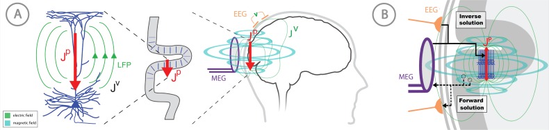
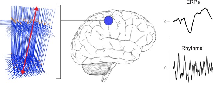
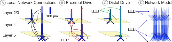
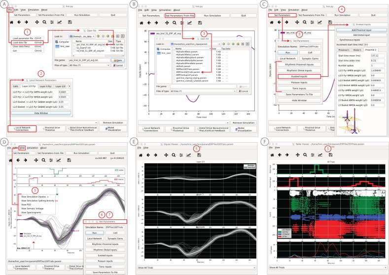
Magneto- and electro-encephalography (MEG/EEG) non-invasively record human brain activity with millisecond resolution providing reliable markers of healthy and disease states. Relating these macroscopic signals to underlying cellular- and circuit-level generators is a limitation that constrains using MEG/EEG to reveal novel principles of information processing or to translate findings into new therapies for neuropathology. To address this problem, we built Human Neocortical Neurosolver (HNN, https://hnn.brown.edu) software. HNN has a graphical user interface designed to help researchers and clinicians interpret the neural origins of MEG/EEG. HNN's core is a neocortical circuit model that accounts for biophysical origins of electrical currents generating MEG/EEG. Data can be directly compared to simulated signals and parameters easily manipulated to develop/test hypotheses on a signal's origin. Tutorials teach users to simulate commonly measured signals, including event related potentials and brain rhythms. HNN's ability to associate signals across scales makes it a unique tool for translational neuroscience research.

Keywords: MEG/EEG; brain rhythms; computational modeling; event related potentials; human; human biology; medicine; neuroscience; thalamocortical system; translational neuroscience.

Figure 1.. Overview of the biophysical origin of MEG/EEG signals and the relationship between HNN and forward/inverse modeling.

(A) HNN bridges the ‘macroscale’ extracranial EEG/MEG recordings to the underlying cellular- and circuit-level activity by simulating the primary electrical currents (J^P) underlying EEG/MEG, which are generated by the postsynaptic, intracellular current flow in the long and spatially-aligned dendrites of a large population of synchronously-activated pyramidal neurons. (B) A zoomed in representation of the relationship between HNN and EEG/MEG forward and inverse modeling. Inverse modeling estimates the location, timecourse and orientation of the primary currents (J^p), and HNN simulates the neural activity creating J^p, at the microscopic scale. Adapted from Jones (2015).

Figure 2.. A schematic illustration of a canonical patch of neocortex that is represented by HNN’s underlying neural model.

(Left) 3D visualization of HNN’s model (pyramidal neurons drawn in blue, interneurons drawn in orange. (Right) Commonly measured EEG/MEG signals (ERPs and low frequency rhythms) from a single brain area that can be studied with HNN.

Figure 3.. Schematic illustrations of HNN’s underlying neocortical network model.

(A) Local Network Connectivity: GABAergic (GABAA/GABAB; lines) and glutamatergic (AMPA/NMDA; circles) synaptic connectivity between single-compartment inhibitory neurons (orange circles) and multi-compartment layer 2/3 and layer five pyramidal neurons (blue neurons). Excitatory to excitatory connections not shown, see Materials and methods. (B) Exogenous proximal drive representing lemniscal thalamic drive to cortex. User defined trains or bursts of action potentials (see tutorials described in text) are simulated and activate post-synaptic excitatory synapses on the basal and oblique dendrites of layer 2/3 and layer five pyramidal neurons as well as the somata of layer 2/3 and layer five interneurons. These excitatory synaptic inputs drive current flow up the dendrites towards supragranular layers (red arrows). (C) Exogenous distal drive representing cortical-cortical inputs or non-lemniscal thalamic drive that synapses directly into the supragranular layer. User defined trains of action potentials are simulated and activate post-synaptic excitatory synapses on the distal apical dendrites of layer 5 and layer 2/3 pyramidal neurons as well as the somata of layer 2/3 interneurons. These excitatory synaptic inputs push the current flow down towards the infragranular layers (green arrows). (D) The full network contains a scalable number of pyramidal neurons in layer 2/3 and layer 5 in a 3-to-1 ratio with inhibitory interneurons, activated by user defined layer specific proximal and distal drive (see Materials and methods for full details).

Figure 4.. An example workflow showing how HNN can be used to link the macroscale current dipole signal to the underlying cell and circuit activity.

The example shown is for a perceptual threshold level tactile evoked response (50% detected) from SI (Jones et al., 2007; see ERP Tutorial text for details). (A) Steps 1 and 2: load data and define the local network structure. (B) Step 3: activate the local network, starting with a predefined parameter set; shown here for the parameter set for perceptual threshold-level evoked response (ERPYes100Trials.param) (C) Step 3 and 4: adjust the evoked input parameters according to user defined hypotheses and simulation experiment, and run the simulation. (D) Step 5: visualize model output; the net current dipole will be displayed in the main GUI window and microcircuit details, including layer-specific responses, cell membrane voltages, and spiking profiles (E and F) are shown by choosing them from the View pull down menu. Parameters can be adjusted to hypothesized circuit changes under different experimental conditions (e.g. see Figure 5).

Figure 4—figure supplement 1.. Sensitivity analysis results of the perceptual threshold level evoked response example showing the relative contribution of each input’s parameters on variance.

Total Sobol indices at each point have been weighted by the std. deviation scaled from 0 to 1.

Figure 5.. Application of HNN to test alternative hypotheses on the circuit level impact of tACS on the somatosensory tactile evoked response (adapted from Sliva et al., 2018).

(A) The early tactile evoked response from above somatosensory cortex before and after 10 min of 10 Hz alternating current stimulation over SI shows that the ~70 ms peak is more prominent in the post-tACS condition. Note that the timing of this peak in the sensor level signal is analogous to the 70 ms peak in the source localized signal in Figure 4B, since the tactile stimulation was the same in both studies and the early signal from SI is similar both at the source and sensor level. (B) HNN was applied to investigate the impact of several possible tACS induced changes in local synaptic efficacy and identify which could account for the observed evoked response data. The parameters in HNN were first adjusted to account for the pre-tACS response using the default HNN parameter set (solid blue line). The synaptic gains between the different cell types was then adjusted through the Set Parameters dialog box to predict that 2x gain in the local inhibitory synaptic weights best accounted for the post-tACS evoked response. (C) Simultaneous viewing of the cell spiking activity further predicted that there is less pyramidal neuron spiking at 70 ms post-tACS, despite the more prominent 70 ms current dipole peak.

Figure 6.. Example spontaneous data from a current dipole source in SI showing transient alpha (~7–14 Hz Hz) and beta (~15–29 Hz) components (data as in Jones et al., 2009).

The data file (‘SI_ongoing.txt’) used to generate these outputs is provided with HNN and plotted through the ‘View → View Spectrograms’ menu item, followed by ‘Load Data’, and then selecting the file. (A) The spectrogram viewer with the default ‘jet’ colormap. (B) The configuration option to change the colormap to other perceptually uniform colormaps, where the lightness value increases monotonically. (C) The spectrogram viewer updated with the perceptually uniform ‘viridis’ colormap.

Figure 7.. An example workflow for simulating alpha frequency rhythm (Jones et al., 2009; Ziegler et al., 2010; see Alpha and Beta Rhythms Tutorial text for details).

(A) Here we are using the default HNN network configuration and not directly comparing the waveform to data, so begin with Step 3: activate the local network. Motivated by prior studies (see text), in this example alpha rhythms were simulated by driving the network with ~10 Hz bursts (presumed to be generated by thalamus) to the local network through proximal and distal projection pathways. The parameter set describing these burst is provided in the Alpha.param file and loaded through the Set Parameters From File button. Adjustable burst drive parameter are shown and here were set with a 50 ms delay between the ~10 proximal and distal drive (red boxes). (B) Step 4: running the simulation with the ‘Run Simulation’ button, shows that a continuous alpha rhythm emerged in the current dipole signal (middle dipole time trace; bottom time-frequency representation). Green and red histograms at the top display the defined distal and proximal burst drive patterns, respectively. (C) Step 5: additional network features, including layer specific power spectral density plots as shown can be visualized through the ‘View’ pull down menu, and compared to data (here compared to the spontaneous SI data shown in Figure 6A). Features of the burst drive can be adjusted (panel A) and corresponding changes in the current dipole signals studied (Steps 6 and 7, see Figure 8).

Figure 8.. An example workflow for simulating transient alpha and beta frequency rhythm as in the spontaneous SI rhythms shown in Figure 6A (Jones et al., 2009; Ziegler et al., 2010; see Alpha and Beta Rhythms Tutorial text for details).

(A) Here we are using the default HNN network configuration and not directly comparing the waveform to data, so begin with Step 3: activate the local network. In this example, a beta component emerged when the parameters of two ~ 10 Hz bursts to the local network through proximal and distal project pathways, as described in Figure 7, were adjusted so that on average they arrived to the network at the same time (see red boxes). This parameter set is provided in the ‘AlphaAndBeta.params’ file. (B) Step 4: running the simulation with the ‘Run Simulation’ button, shows that intermittent and transient alpha and beta rhythms emerge in the current dipole signal (middle dipole time trace; bottom time-frequency representation). Green and red histograms at the top display the defined distal and proximal burst drive patterns, respectively. Due to the stochastic nature of the bursts, on some cycles of the drive, the distal burst was simultaneous with the proximal burst and strong enough to push current flow down the dendrites to create a beta event (see red box). This model derived prediction reproduced several features of the data, including alpha and beta peaks in the corresponding PSD that were more closely matched to the recorded data (C). Model predictions were subsequently validated with invasive recordings in mice and monkeys (Sherman et al., 2016; see further discussion in text).

Figure 9.. An example workflow for simulating canonical pyramidal-interneuron gamma (PING) rhythms (Lee and Jones, 2013; see Gamma Rhythms Tutorial text for details).

(A) Here we are using the default HNN network configuration (with some parameter adjustments as shown in panel B) and we are not directly comparing the waveform to data, so begin with Step 3: activate the local network. Motivated by prior studies on PING mechanisms (see text), in this example PING rhythms were simulated by driving the pyramidal neuron somas with noisy excitatory synaptic input following a Poisson process. The parameters defining this noisy drive are viewed and adjusted through the Set Parameters button as shown, see text and Materials and methods for parameter details. This parameter set for this example is provided in the ‘gamma_L5weak_L2weak.param’ file. In this example, all synaptic connections within the network are turned off (synaptic weight = 0), except for reciprocal connections between the excitatory (AMPA only) and inhibitory (GABAA only) cells within the same layer. The local network connectivity can be viewed and adjusted through the Set Network Connection button or pull down menu, as shown in (B). (C) Step 4: running the simulation with the ‘Run Simulation’ button, shows that a ~ 50 Hz gamma rhythm is produced in the current dipole signal (middle dipole time trace; bottom time-frequency representation). The black histogram at the top displays the noisy excitatory drive to the network. (D–F) Step 5: additional network features, including cell spiking responses, somatic voltages, and layer specific power spectral density plots as shown can be visualized through the ‘View’ pull down menu.

Figure 10.. An example simulation describing how parameter adjustments to the canonical PING mechanism can account for source localized visually-induced gamma rhythms recorded with MEG.

(A) An example single trial current dipole waveform generated from a stationary square-wave grating, presented from 0 to 700 ms. MEG data was source localized to the pericalcarine region of the visual cortex (top). The corresponding time-frequency representation (bottom) shows transient bursts of induced gamma activity (bottom). Data is as in Pantazis et al. (2018) and described further in text. (B) Analogous waveforms from 100 trials overlaid (top) and corresponding averaged time-frequency spectrograms (bottom). Averaging in the spectral domain creates the appearance of a more continuous oscillation. (C) Parameters used to simulate the canonical PING rhythm in Figure 9 were adjusted (Steps 6 and 7) to test the hypothesis that a reduced rate of Poisson synaptic input to the pyramidal neurons could account for the bursty nature of the observed gamma data. The parameter set for this example is provided in the ‘gamma_L5weak_L2weak_bursty.param’ file. In this example, the Poisson input rates to the Layer 2/3 and Layer 5 cells were reduced to 4 Hz and 5 Hz, respectively, and the NMDA synaptic inputs were set to a small positive weight (dialog box not shown). Running the simulation will display a histogram of the Poisson drive (top), the current dipole waveform (middle), and the corresponding time-frequency spectrogram (bottom). With this parameter adjustment,~50 Hz bursty gamma activity is reproduced. A scaling factor of 5 was applied to the net current dipole to produce a signal amplitude comparable to the data (<0.1 nAm), suggesting that only ~1000 pyramidal neurons contributed the recorded signal. (D) Poisson input over 100 simulations (top), current dipole waveforms overlaid (middle), and the corresponding spectrogram average (bottom). Similar to the recorded data, averaging in the spectral domain creates the appearance of a more continuous oscillation. (E–F) Microcircuit details including cell spiking responses and layer specific current dipoles shows Layer 5 activity dominates the net current dipole signal, see text for further description.

Figure 11.. Example of the ERP parameter optimization procedure for a suprathreshold tactile evoked response.

(A) Source localized SI data from a suprathreshold tactile evoked response (100% detection; purple) is shown overlaid with the corresponding HNN evoked response (black) using the threshold level evoked response parameter set detailed in Figure 4, as in initial parameter set. The RMSE between the data and the model is initially high at 30.53. (B) To improve the fit to the data, a procedure for sequentially optimizing the strengths of the proximal and distal drive inputs generating the evoked response can be run. The ‘Configure Optimization’ option is available under the ‘Simulation’ pull down menu. A dialog box allows users to choose and set a range over free optimization parameters, see text for details. (C) The GUI displays an intermediate fit after the first optimization step, specific to the first proximal drive. (D) The final fit is displayed once the optimization is complete. Here, the simulation from the optimized parameter set for the suprathreshold evoked response is shown in gray with an improved RMSE of 15.54 compared to 30.53 for the initial model. See Figure 11—figure supplements 1 and 2 for a further description of the optimization routine and parameter sensitivity analysis.

Figure 11—figure supplement 1.. Weighted scoring of the stepwise optimization procedure for suprathreshold level evoked response example, see text for details.

(A) Probability distribution of input timing for each input. (B) Corresponding cumulative distribution as a contribution index. (C) Unique Contribution Index that is reduced by subsequent input’s CDFs. (D) Extended Contribution Index in which the subtracted CDFs are subject to a decay factor.

Figure 11—figure supplement 2.. Sensitivity analysis results of the suprathreshold level evoked response example showing the relative contribution of each input’s parameters on variance.

Total Sobol indices at each point have been weighted by the std. deviation scaled from 0 to 1.

References

1. Alexanderian A, Gremaud PA, Smith RC. Variance-based sensitivity analysis for time-dependent processes. Reliability Engineering & System Safety. 2020;196:106722. doi: 10.1016/j.ress.2019.106722. - DOI
1. Badre D, Frank MJ, Moore CI. Interactionist neuroscience. Neuron. 2015;88:855–860. doi: 10.1016/j.neuron.2015.10.021. - DOI - PubMed
1. Bannister AP. Inter- and intra-laminar connections of pyramidal cells in the neocortex. Neuroscience Research. 2005;53:95–103. doi: 10.1016/j.neures.2005.06.019. - DOI - PubMed
1. Barrès V, Simons A, Arbib M. Synthetic event-related potentials: a computational bridge between neurolinguistic models and experiments. Neural Networks. 2013;37:66–92. doi: 10.1016/j.neunet.2012.09.021. - DOI - PubMed
1. Bekkers JM. Properties of voltage-gated potassium currents in nucleated patches from large layer 5 cortical pyramidal neurons of the rat. The Journal of Physiology. 2000;525:593–609. doi: 10.1111/j.1469-7793.2000.t01-1-00593.x. - DOI - PMC - PubMed
Publication types