The Use of Dijkstra's Algorithm in Assessing the Correctness of Imaging Brittle Damage in Concrete Beams by Means of Ultrasonic Transmission Tomography

Abstract

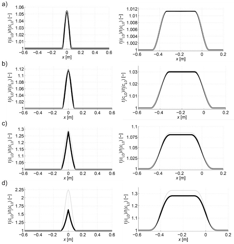
The accuracy of transmission ultrasonic tomography for the detection of brittle damage in concrete beams can be effectively supported by the graph theory and, in particular, by Dijkstra's algorithm. It allows determining real paths of the fastest ultrasonic wave propagation in concrete containing localized elastically degraded zones at any stage of their evolution. This work confronts this type of approach with results that can be obtained from non-local isotropic damage mechanics. On this basis, the authors developed a method of reducing errors in tomographic reconstruction of longitudinal wave velocity maps which are caused by using the simplifying assumptions of straightness of the fastest wave propagation paths. The method is based on the appropriate elongation of measured propagation times of the wave transmitted between opposite sending-receiving transducers if the actual propagation paths deviate from straight lines. Thanks to this, the mathematical apparatus used typically in the tomography, in which the straightness of the fastest paths is assumed, can be still used. The work considers also the aspect of using fictitious wave sending-receiving points in ultrasonic tomography for which wave propagation times are calculated by interpolation of measured ones. The considerations are supported by experimental research conducted on laboratory reinforced concrete (RC) beams in the test of three-point bending and a prefabricated damaged RC beam.

Keywords: concrete; damage mechanics; damage parameter; elastic degradation; experimental research; graph theory; internal length; non-destructive testing; ultrasonic tomography.

Figure 1

Scheme of a cell system, transmitting/receiving points, and rays in a plane area examined tomographically.

Figure 2

Distribution of the weight function $\psi$ for $x=0$.

Figure 3

Shape of concrete specimens for the tension tests (based on Reference [34]).

Figure 4

(a) Comparison of relations $P_{\exp }$-$u_{\exp }$ and $P$-$u$ using 121 finite elements. (b) Comparison of relations $P$-$u$ using 121 and 241 finite elements.

Figure 5

Calculated distributions of $D$ during the development of the damaged zone in the middle of the specimen: (a) model of the specimen $d\times h=20$ cm $\times 30$ cm (b) specimen model with twice the total width and length increased $d\times h$ $=40$ cm $\times 60$ cm ($d$, $h$ according to Figure 3).

Figure 6

Relative changes of Young’s modulus (a) and longitudinal wave velocities (b) for distributions of $D$ from Figure 5b.

Figure 7

Illustrative orthogonal node arrangement for a graph in a plane problem (based on Reference [42]).

Figure 8

Scheme of the beam model with the assumed damage distribution and the system of transmitting/receiving points and rays.

Figure 9

The shape of the paths of the fastest propagation between the selected transmitting/receiving points in the longitudinal section of the beam with the area damaged at $\min \left(E_{\mathrm{D}}/E_0\right)=0.2$ and ${\mathsf{\Delta }}_{\mathrm{n}}\approx$ (a) $100$ mm, (b) $50$ mm, (c) $25$ mm, (d) $12.5$ mm, (e) $6.25$ mm, and (f) $3.125$ mm.

Figure 10

The shape of paths of the fastest propagation between the selected transmitting/receiving points in the longitudinal section of the beam depending on the degree of elastic degradation in the damaged zone $\min \left(E_{\mathrm{D}}/E_0\right)=$ (a) 0.9, (b) 0.8, (c) 0.6, and (d) 0.2 (for ${\mathsf{\Delta }}_{\mathrm{n}}=3.125$ mm).

Figure 11

Times of wave propagation $t_{\mathrm{path},i}$ on the fastest paths, and $t_{\mathrm{ray},i}$ over the straight rays between the transmitting/receiving points in the different phases of the defect evolution: $\min \left(E_{\mathrm{D}}/E_0\right)=$ (a) 0.9, (b) 0.8, (c) 0.6, and (d) 0.2. The results are presented as a function of the position of the transmitting points: a black line for the fastest paths determined by Dijkstra’s algorithm (for ${\mathsf{\Delta }}_{\mathrm{n}}=3.125$ mm); a grey line for the paths established as straight rays. The diagrams on the left refer to the paths connecting the opposite points and those on the right to the points lying diagonally at an angle of $45°$ to each other in relation to the axis $x$.

Figure 12

Propagation times $t_{\mathrm{path},i}$, $t_{\mathrm{ray},i}$ and $t_{\mathrm{ray}\mathrm{approx},i}$ between the opposite transmitting/receiving points for a defect with $\min \left(E_{\mathrm{D}}/E_0\right)=0.2$. $t_{\mathrm{ray}\mathrm{approx},i}$ were calculated according to relation (22) with $\beta ={\beta }_{\mathrm{opt}}$.

Figure 13

Originally assumed distributions of wave velocity in the longitudinal section of the beam in different stages of defect evolution (a) and their tomographic reconstructions according to Equation (3): (b) calculated using the propagation times $t_{\mathrm{ray},i}=t_{\mathrm{ray}\mathrm{approx},i}$ for the paths connecting the opposite points and $t_{\mathrm{ray},i}=t_{\mathrm{path},i}$ for the paths connecting the points diagonally, (c) calculated using only the propagation times $t_{\mathrm{ray},i}=t_{\mathrm{path},i}$ (red dotted lines—explanation in the text).

Figure 14

Times of wave propagation $t_{\mathrm{path},i}$ and $t_{\mathrm{path}\mathrm{int},i}$ on the fastest paths between transmitting/receiving points in different phases of defect evolution: $\min \left(E_{\mathrm{D}}/E_0\right)=$ (a) 0.9, (b) 0.8, (c) 0.6, and (d) 0.2. The results are presented as a function of the position of the transmitting points: a black line for the fastest paths determined by Dijkstra’s algorithm (for ${\mathsf{\Delta }}_{\mathrm{n}}=3.125$ mm); a grey line in case of interpolation with nodes marked with circles. The diagrams on the left refer to the paths connecting the opposite points and those on the right to the points lying diagonally at an angle of $45°$ to each other in relation to the axis $x$.

Figure 15

Propagation times $t_{\mathrm{path},i}$, $t_{\mathrm{ray},i}$ and $t_{\mathrm{ray}\mathrm{approx},i}$ between the opposite transmitting/receiving points for a defect with $\min \left(E_{\mathrm{D}}/E_0\right)=0.2$. $t_{\mathrm{ray}\mathrm{approx},i}$ were calculated according to relation (28) with $\beta ={\beta }_{\mathrm{opt}}$.

Figure 16

Tomographic reconstructions of the wave velocity distribution from Figure 13a according to Equation (3): (a) calculated with the propagation times $t_{\mathrm{ray},i}=t_{\mathrm{ray}\mathrm{approx},i}$ for the paths connecting the opposite points and $t_{\mathrm{ray},i}=t_{\mathrm{path}\mathrm{int},i}$ for the paths connecting the points diagonally, (b) calculated only with the propagation times $t_{\mathrm{ray},i}=t_{\mathrm{path}\mathrm{int},i}$ (red dotted lines—explanation in the text).

Figure 17

Flowchart of the calculation process.

Figure 18

Scheme of the beams and the assumed system of transmitting/receiving points and rays.

Figure 19

(a) Beam loading scheme. (b) Illustrative pictures of beam No. 3 before and after an action of cracking load.

Figure 20

Propagation times $t_{\mathrm{path}\mathrm{int},i}$ and $t_{\mathrm{ray}\mathrm{approx},i}$ between the transmitting/receiving points in the beams before and after an action of cracking load: (a) No. 1, (b) No. 2, and (c) No. 3. The results are presented as a function of the position of the transmitting points: $t_{\mathrm{path}\mathrm{int},i}$ a grey line with nodes marked with circles, and $t_{\mathrm{ray}\mathrm{approx},i}$ a black, dashed line. The diagrams on the left refer to the paths connecting the opposite points and those on the right to the points lying diagonally at an angle of $45°$ and $135°$ to each other in relation to the axis $x$.

Figure 21

Example of signal recorded by the receiving head (transmitting point No. 4 and receiving point No. 3 in beam No. 3): (a) before load; (b) after an action of cracking load.

Figure 22

Tomographic reconstructions of the distribution of wave velocity according to Equation (3) in the longitudinal section of the beam before and after an action of the cracking load: (a) No. 1, (b) No. 2, and (c) No. 3 (red dotted lines—explanation in the text).

Figure 23

Scheme of the beam and the assumed system of transmitting/receiving points and rays.

Figure 24

(a) Picture of the beam (the places of visible cracks are marked with the slats put on the upper surface of the beam). (b) Shape and width of the visible cracks.

Figure 25

Propagation times $t_{\mathrm{path}\mathrm{int},i}$ and $t_{\mathrm{ray}\mathrm{approx},i}$ between the transmitting/receiving points in the beam. The results are presented as a function of the position of the transmitting points: $t_{\mathrm{path}\mathrm{int},i}$ grey lines with nodes marked with circles, and $t_{\mathrm{ray}\mathrm{approx},i}$ a black dashed line. The top diagram refer to the paths connecting the opposite points and the bottom one to the points lying diagonally at an angle of $63.4°$ and $116.6°$ to each other in relation to the axis $x$.

Figure 26

Example of a signal recorded by the receiving head (transmitting point No. 3 and receiving point No. 1).

Figure 27

Tomographic reconstructions of the distribution of wave velocity according to Equation (3) in the longitudinal section of the beam (red dotted line—explanation in the text).

References

1. Drobiec Ł., Jasiński R., Piekarczyk A. Diagnostyka Konstrukcji Żelbetowych. PWN; Warsaw, Poland: 2010. (In Polish)
1. Jacobs F. Durability of concrete in structural members. Beton-und Stahlbetonbau. 2019;114:383–391. doi: 10.1002/best.201900003. - DOI
1. Breysse D., Balayssac J.P., Biondi S., Corbett D., Goncalves A., Grantham M., Luprano V.A.M., Masi A., Monteiro A.V., Sbartai Z.M. Recommendation of RILEM TC249-ISC on non destructive in situ strength assessment of concrete. Mater. Struct. 2019;52:71. doi: 10.1617/s11527-019-1369-2. - DOI
1. Bai Y., Basheer M., Cleland D., Long A. State-of-the-art applications of the pull-off test in civil engineering. Int. J. Struct. Eng. 2009;1:93–103. doi: 10.1504/IJSTRUCTE.2009.030028. - DOI
1. Dillon R., Rankin G.I.B. Cube, cylinder, core and pull-off strength relationships. Proc. Inst. Civ. Eng. Struct. Build. 2013;166:521–536. doi: 10.1680/stbu.11.00075. - DOI
LinkOut - more resources