Cognitive control and automatic interference in mind and brain: A unified model of saccadic inhibition and countermanding

Abstract

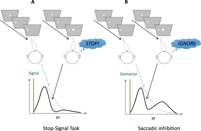
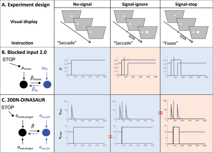
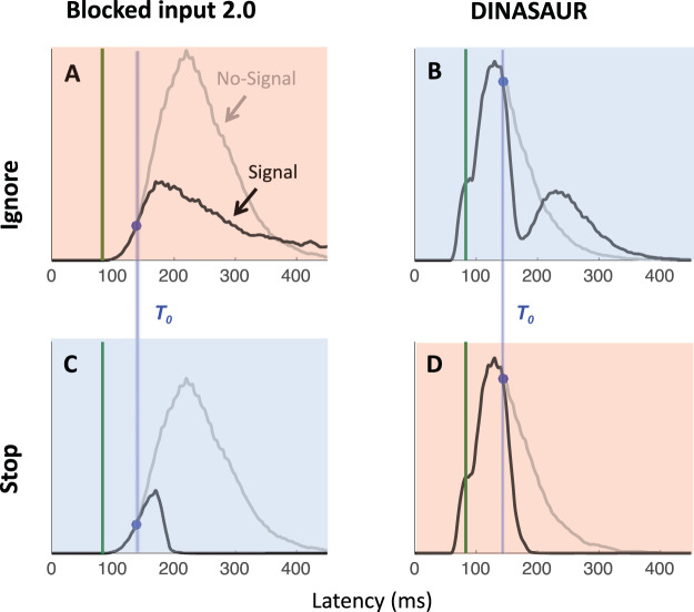
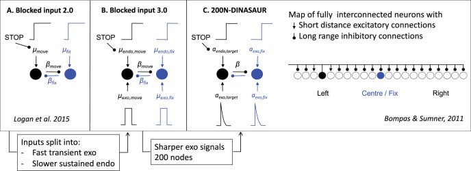
Countermanding behavior has long been seen as a cornerstone of executive control-the human ability to selectively inhibit undesirable responses and change plans. However, scattered evidence implies that stopping behavior is entangled with simpler automatic stimulus-response mechanisms. Here we operationalize this idea by merging the latest conceptualization of saccadic countermanding with a neural network model of visuo-oculomotor behavior that integrates bottom-up and top-down drives. This model accounts for all fundamental qualitative and quantitative features of saccadic countermanding, including neuronal activity. Importantly, it does so by using the same architecture and parameters as basic visually guided behavior and automatic stimulus-driven interference. Using simulations and new data, we compare the temporal dynamics of saccade countermanding with that of saccadic inhibition (SI), a hallmark effect thought to reflect automatic competition within saccade planning areas. We demonstrate how SI accounts for a large proportion of the saccade countermanding process when using visual signals. We conclude that top-down inhibition acts later, piggy-backing on the quicker automatic inhibition. This conceptualization fully accounts for the known effects of signal features and response modalities traditionally used across the countermanding literature. Moreover, it casts different light on the concept of top-down inhibition, its timing and neural underpinning, as well as the interpretation of stop-signal reaction time (RT), the main behavioral measure in the countermanding literature. (PsycInfo Database Record (c) 2020 APA, all rights reserved).

Figure 1

Typical design (above) and results (below) in the saccadic stop-signal task (SST, panel A) and saccadic inhibition (SI, panel B) paradigms. Both paradigms involve a stimulus jump from center to periphery, sometimes followed by the onset of a central signal (right subpanels above, black lines below), sometimes not (left subpanels, gray lines). The signal onset time is indicated by vertical green lines and the delay between the target jump and the signal is referred to as the stimulus onset asynchrony (SOA). The two tasks differ in the instruction associated with the signal onset: withhold the saccade in the SST, ignore the signal and perform the saccade in the SI. A. Instructions to stop remove slower responses from the RT distribution, but fast responses escape (“failed stops”). B. The same visual events associated with an ignore instruction typically produce a dip in the latency distribution, where saccades are delayed and subsequently recover, so that the total number of saccades are about the same between signal present and no-signal distributions. We propose that on trials where participants are told to stop their saccade in response to the signal onset (A), the initial reduction in saccade probability has the same automatic source and therefore will happen at the same time as the dip in the ignore condition (B), but the recovery from the dip will be diminished or absent due to later top-down inhibition.

Figure 2

Inputs to blocked input 2.0 and 200N-Dinasaur for each task condition, based on published versions (blue shaded areas; Bompas & Sumner, 2011; Logan et al., 2015) or parsimonious generalizations to new conditions (red shaded areas, using SOA = 83 ms as in the new experiments introduced below). A. Schematic task conditions (see Figure 1 for description). B. Blocked input 2.0 was originally designed for the stop task encompassing the no-signal and signal-stop conditions (blue shade). In the most parsimonious generalization to the ignore instructions (red shade), the late “blocking” of move input does not occur (black line), just as in no-signal conditions, while the stimulus onset reactivates fixation input (blue line) just as in the signal-stop condition. C. 200N-DINASAUR was shown to capture saccadic inhibition (no-signal = prosaccade; signal-ignore = distractor condition; blue shade). Out of the 200 nodes, here only the fixation and target nodes are shown. The model categorizes inputs as exogenous (stimulus-elicited and transient, upper plots) or endogenous (instruction-related and sustained, lower plots). A straightforward generalization to the stop instruction (red shade) is to assume the exogenous inputs are unchanged, while the endogenous input switches from the target back to fixation, like in blocked input 2.0. Note that in blocked input 2.0, this switch is not simultaneous: Fixation drive reappears before move drive is blocked to allow for the extra rapidity of a stimulus-driven response. In DINASAUR, the exogenous input already accounts for the rapid stimulus-elicited activity, so parsimoniously the endogenous switch can be simultaneous: The onset of endogenous fixation drive is given the same delay as the offset of endogenous saccade drive. SOA = stimulus onset asynchrony.

Figure 3

Simulated RT distributions from 10,000 trials using blocked input 2.0 (A, C) and 200N-DINASAUR (B, D) for signal onset (green line) at SOA 83 ms. Blue shaded areas indicate those instantiations of each models as published. Red shaded areas indicate predictions for new conditions based on the assumptions described in Figure 2. The DINASAUR model (with blocked input for stopping) captures well the typical pattern of results obtained in both paradigms. Blocked input 2.0 (with automatic fixation activity for ignore conditions) is not able to produce the sharp dips expected from the saccadic inhibition literature (but see blocked input 3.0 and Figures 4–5). Both models predict a perfect alignment across instructions of the time when the signal RT distribution (black) departs from the no-signal RT distribution (gray), indicated by the blue dots (T₀) and highlighted by blue vertical bars. Note that the difference in mean and variance of the RT distributions between the models simply reflects the parameters inherited from previous publications; they have never been fitted to the same behavioral distributions. Relatedly, the position of T₀ (blue dots) relative to the baseline distribution merely depends on where that distribution lies relative to signal onset (the SOA). The important aspect here is generalization ability of each model across instructions.

Figure 4

Overview of models and their relationships. A. Blocked input 2.0 as in Logan et al. (2015). B. Blocked input 3.0 integrates aspects of DINASAUR into blocked input 2.0 in an attempt to capture the signal-ignore condition. Its inputs are split into two conceptually different streams: A fast and transient drive tied to visual onsets (exogenous) and a slower sustained drive tied to instructions (endogenous). C. 200N-DINASAUR is a map of fully interconnected neurons representing part of the left, central, and right visual fields, invented to capture simplified SC dynamics. The temporal dynamics of its exogenous signals (quick growth and exponential decay) is a key factor for creating sharp dips and quick recovery.

Figure 5

Inputs and simulations from blocked input 3.0 and 3.1. A–B. In the most straightforward generalization from blocked input 2.0, we assume in blocked input 3.0 that the transient visual signals associated with signal onset are the same size as the original fixation inputs in blocked input 2.0 (discontinuous blue line). Blocked input 3.1 assumes that the transient activity from the signal is larger (in this case three times higher) than the baseline fixation amplitude (continuous blue line). C. Simulated RT for blocked input 3.0 shows some dip, but this remains very shallow. D. The stop condition for blocked input 3.0 is the same as for blocked input 2.0. E–F. Simulated RTs for blocked input 3.1 now show a clear dip and recovery as expected in the signal-ignore condition (E), while still capturing the signal-stop condition (F).

Figure 6

A–C. Mean firing rates from 1,000 simulated trials using each model under the stop condition, at the target and fixation nodes. The solid green line indicates the signal onset, here chosen at stimulus onset asynchrony (SOA) 133, matching the experiments presented in the Empirical data - Results section. The dashed green line shows the divergence time, that is, the time at which this signal starts having an effect on the neuronal map, while the black vertical line indicates the stop signal reaction time (SSRT), estimated from the simulated RT from each model. Activity was averaged across trials leading to successful inhibition (black and dark blue lines, signal-inhibit trials) and compared with “latency matched” no-signal trials (gray and light blue lines; i.e., no-signal trials in which latency is greater than SOA + non-decision time). On the y-axis for the target node, Th indicates the saccade initiation threshold (although this is not directly relevant for average firing rates, see text). D. Mean growth and decay rates from frontal eye field (FEF) neurons and simulations from each model (BI2 and BI3 refer to blocked input 2.0 and 3.1, respectively), using the same format as Figure 14 in Logan et al. (2015).

Figure 7

A. Latency distributions for Participant 1 in Experiment 1 across SOAs (rows) in the ignore and stop contexts. Gray lines indicate distributions in which no signal was presented. Black lines indicate distributions of trials in which a signal occurred. Blue dots indicate the dip onset (i.e., where the two distributions first diverge); red dots show dip maximum. B. Green indicate the only data used for fitting the DINASAUR model: dip onsets from the ignore condition after pooling across all SOAs, no-signal distributions from the ignore and stop contexts, and the proportion of failed stops at SOA 50. Red lines show the fitted no-signal distributions for this participant (see the “Modeling Results” section for modeling details). C. Simulated RT distributions across all conditions for this participant. D. Observed (points) versus simulated (red lines) key measures at each SOA: dip onset in the ignore and stop conditions, proportion of failed stops and SSRT, all in ms (see Figures A4–A7 for all individual data).

Figure 8

A–C. Dip onset times (T₀) for each participant in the ignore (open circles) and stop (stars) contexts of each experiment, along with regression lines across SOAs on each condition. As predicted, dip onsets are locked on signal onset and are temporally aligned between the ignore and stop contexts, consistently across experiments. D–F. Overlap of dip timing between the ignore and stop contexts in each experiment, highlighted by blue vertical bars. Distributions show saccade latency locked on signal onset, allowing pooling of trials across the SOAs to best visualize the timing of dip onset (blue dots) and maximum (red).

Figure 9

Traditional stop signal task measures from observed and simulated data. A–B. Proportion of failed stops (A) and stop signal RT (SSRT, B) across SOAs, from the pooled data across observers (black diamonds) and in DINASAUR simulations (red lines) with and without failure (continuous and dotted lines). The SSRT was calculated using the integration method (Verbruggen et al., 2013). C. Cumulative distributions for observed no-signal (light gray) and signal trials (black continuous, semidashed, dashed, and dotted for SOA 50, 83, 133, and 183, respectively). D. Same as C for DINASAUR simulation (with failure), also pooled across observers. See Figures A5–A7 in Appendix A for individual data and Figure A9 for scaled cumulative distributions.

Figure 10

Distributions of RT locked on signal onset, pooled across all SOAs and observers, along with simulations using 200N-DINASAUR model pooled in the same way. Same conventions as Figure 8.

Figure A1

Latency distributions for each participant (columns) and stimulus onset asynchrony (SOA; rows) in the ignore and stop contexts of Experiment 1. Green lines indicate the signal onset. Gray lines indicate distributions in which no signal was presented. Black lines indicate distributions of trials in which a signal occurred. Blue dots indicate the dip onset (i.e., where the distributions diverge, not necessarily where one takes a down-turn); red dots show dip maximum.

Figure A2

Same as A2 for Experiment 2. As expected, strategic adjustments across conditions were particularly large in Experiment 2 (where the two contexts were kept fully separated) and meant the visual signal often arrived too late to have much effect, especially for the fastest participants (P1 and P4). Nevertheless, when dips were observed in both contexts, Experiment 2 confirmed the results from Experiment 1. SOA = stimulus onset asynchrony.

Figure A3

Same as A1 for Experiment 3 after pooling data from white and dark signals. SOA = stimulus onset asynchrony.

Figure A4

Individual T₀ at each SOA in the ignore (circles) and stop instructions (stars) along with simulated T₀ using the ignore (dashed lines) and stop (continuous line) parameters from Appendix E. Missing points and lines indicate cases when the observed or simulated data did not show dips. Even though we only use T_0p from the ignore condition to constrain the model, note how well the model generalizes to each stimulus onset asynchrony (SOA) and across instructions.

Figure A5

Observed data in the stop task (gray and black) along with model simulations (red). A. Cumulative distribution of no-signal RT (gray and dark red) and signal RT for SOAs 50, 83, and 133 (continuous, semidashed, and dashed black lines, respectively, for observed data and bright red lines for model). B–C. Inhibition function and stop signal reaction time (SSRT) for observed (diamonds) and simulated (lines) stop-signal data. RT = reaction time; SOA = stimulus onset asynchrony.

Figure A6

Same as A5 for Experiment 2. RT = reaction time; SSRT = stop signal reaction time; SOA = stimulus onset asynchrony.

Figure A7

Same as A5 for Experiment 3. RT = reaction time; SSRT = stop signal reaction time; SOA = stimulus onset asynchrony.

Figure A8

DINASAUR accounts for patterns in neural activity previously taken to imply independence of go and stop processes. A and C. Mean simulated activity during unsuccessful stop trials (signal-respond) and latency matched no-signal trials at stimulus onset asynchrony (SOA) 83 ms, using the same convention as Figure 6 and matching Figure 4A and C in Boucher, Palmeri, et al. (2007). B. Same data as in A but locked on saccade onset, following Figure 3F in Paré and Hanes (2003). D. Same data as in C but locked on saccade onset (not shown in Paré & Hanes, 2003, shown here for completion). Green shades indicate those time windows chosen in these two previous articles to illustrate the equality of neural activity between signal-respond and fast no-signal trials. Clear differences are apparent outside these time windows.

Figure A9

Cumulative distributions of failed-stops, scaled to represent frequency rather than number of responses, for no-signal (light gray) and signal trials (black continuous, semidashed and dashed for stimulus onset asynchrony (SOA) 50, 83, and 133, respectively; same conventions as Figure 9C–D). The expected “temporal ordering” of scaled distributions (with the shortest SOA most on the left and the no-signal condition most on the right) is apparent in their early part. However, the bimodality in failed-stops distributions, diagnostic of trigger failures, breaks this pattern, as error curves shift to the right of the no-signal curve after the dip (see the Nonindependence of Go and Stop Processes section in Discussion for the implications of such pattern). Scaled representations may be misleading because, for the least populated categories (errors at short SOA), the fastest responses appear to occur earlier compared to fastest responses of the more populated categories (longer SOA or no-signal). Nonscaled representations show this not to be the case.

References

1. Akerfelt A., Colonius H., & Diederich A. (2006). Visual-tactile saccadic inhibition. Experimental Brain Research, 169, 554–563. 10.1007/s00221-005-0168-x - DOI - PubMed
1. Armstrong I. T., & Munoz D. P. (2003). Inhibitory control of eye movements during oculomotor countermanding in adults with attention-deficit hyperactivity disorder. Experimental Brain Research, 152, 444–452. 10.1007/s00221-003-1569-3 - DOI - PubMed
1. Asrress K. N., & Carpenter R. H. S. (2001). Saccadic countermanding: A comparison of central and peripheral stop signals. Vision Research, 41, 2645–2651. 10.1016/S0042-6989(01)00107-9 - DOI - PubMed
1. Band G. P. H., van der Molen M. W., & Logan G. D. (2003). Horse-race model simulations of the stop-signal procedure. Acta Psychologica, 112, 105–142. 10.1016/S0001-6918(02)00079-3 - DOI - PubMed
1. Bissett P. G., & Logan G. D. (2014). Selective stopping? Maybe not. Journal of Experimental Psychology: General, 143, 455–472. 10.1037/a0032122 - DOI - PMC - PubMed
Publication types