Integrating Computational Methods to Investigate the Macroecology of Microbiomes

Abstract

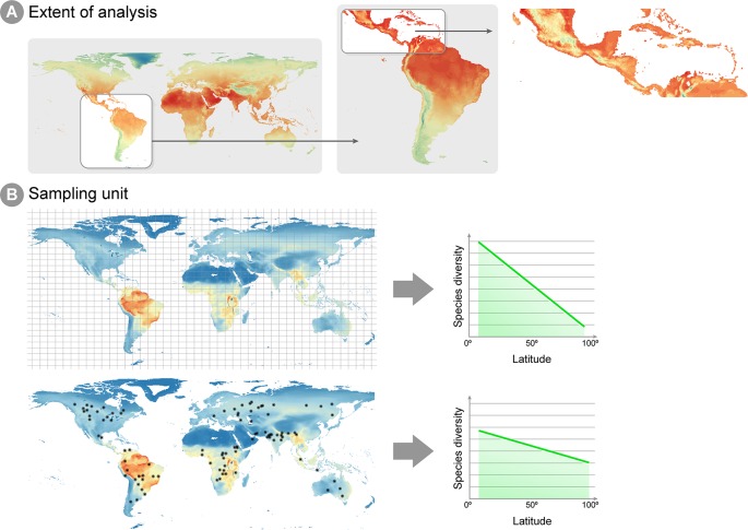
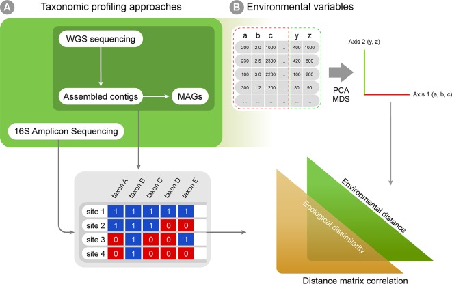
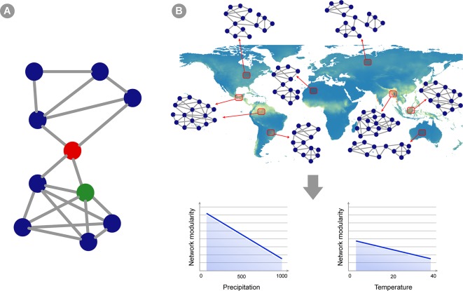
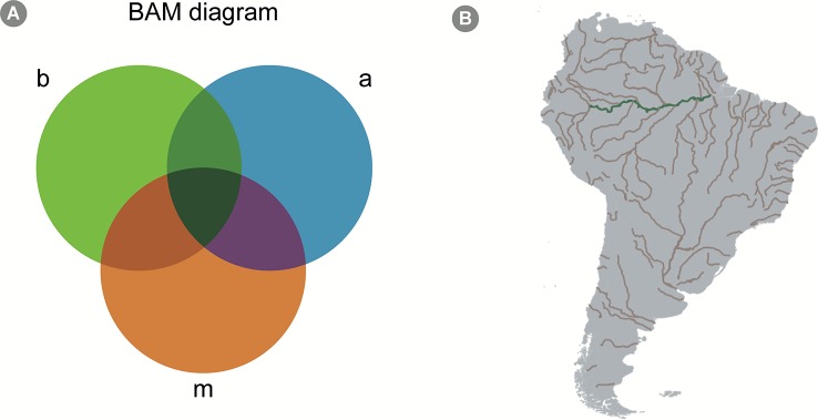
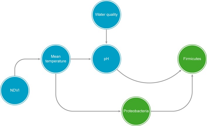
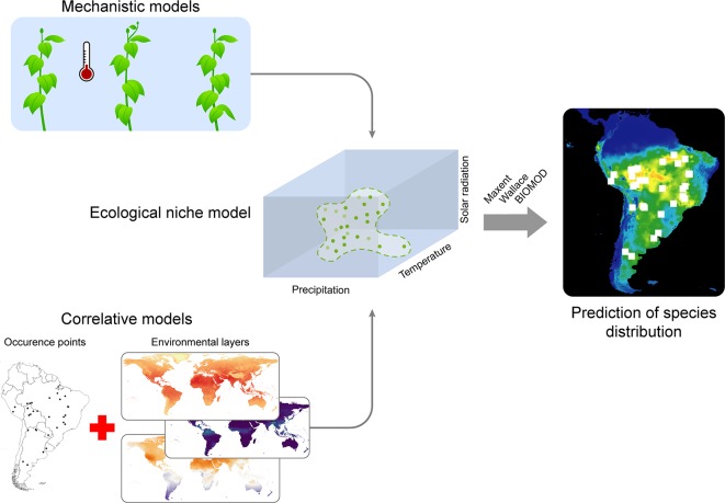
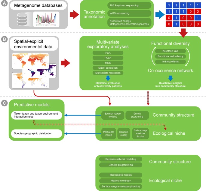
Studies in microbiology have long been mostly restricted to small spatial scales. However, recent technological advances, such as new sequencing methodologies, have ushered an era of large-scale sequencing of environmental DNA data from multiple biomes worldwide. These global datasets can now be used to explore long standing questions of microbial ecology. New methodological approaches and concepts are being developed to study such large-scale patterns in microbial communities, resulting in new perspectives that represent a significant advances for both microbiology and macroecology. Here, we identify and review important conceptual, computational, and methodological challenges and opportunities in microbial macroecology. Specifically, we discuss the challenges of handling and analyzing large amounts of microbiome data to understand taxa distribution and co-occurrence patterns. We also discuss approaches for modeling microbial communities based on environmental data, including information on biological interactions to make full use of available Big Data. Finally, we summarize the methods presented in a general approach aimed to aid microbiologists in addressing fundamental questions in microbial macroecology, including classical propositions (such as "everything is everywhere, but the environment selects") as well as applied ecological problems, such as those posed by human induced global environmental changes.

Keywords: co-occurrence networks; machine learning; microbial community modeling; microbial macroecology; spatial scales.

Figure 1

Spatial extent and sampling unit in macroecological analyses. (A) Different spatial extents can be analyzed in a macroecological study, which will reflect on the environmental information available for inference and how much extrapolation can be derived from the conclusions of the study. The figure shows annual mean temperature per cell, ranging from low temperatures in blue and high temperatures in red. Notice that the lowest temperatures (blue and green cells) are different for each extent. For instance, when studying Central America, the lowest temperatures can be found in Mexico highlands, whereas an extent focused on the whole Neotropics show lowest temperatures around the Andes mountains. Therefore, caution is necessary when inferences from studies on the Central America are extrapolated to the Neotropics extent. (B) Example of two different sampling units in macroecological studies: equally distant squared grids and local sites unevenly distributed through the globe. As highlighted by Hillebrand (2004), squared grids consist of a value averaged across sites within the grid, which decreases the effect of local scale factors (e.g., biotic interactions, dispersal and stochasticity) on the latitude gradient diversity pattern.

Figure 2

A workflow summary for taxonomic annotation and exploratory analyses. Taxonomic annotation methods are used to generate, for instance, presence-absence matrices (A), which can be combined with environmental variables into correlation analyses (B). The biological variation in environmental variables can be simplified through ordination analyses (such as PCA and MDS). Finally, distance matrices can be created for both ecological and environmental variation, and distance matrix correlation can be used to infer if environmental distances correlate with ecological differences among sampling sites.

Figure 3

Co-occurrence networks applied to microbial macroecology. (A) A hypothetical example of a co-occurrence network. Circles represent different taxa and edges connecting two circles indicate statistically significant co-occurrence between those two taxa, i.e., they co-occur more than expected by chance in the set of samples analyzed. Network structure can indicate ecosystem properties, and these can be translated into statistics summarizing network topology (see Box 1). For instance, this hypothetical network shows two subunits (or modules) separated by the taxon indicated as a red circle. This taxon is also a node with high betweenness centrality (i.e., indirect connections between any two nodes in the network has a high probability of going through this node), whereas the green circle represents a node with high degree (i.e., showing a connection to many other taxa). (B) A hypothetical example of a macroecological study using co-occurrence networks. Red squares represent an area where several samples were gathered and analyzed, yielding a single abundance matrix and a corresponding co-occurrence network (two sites pointing to the same network represent areas in which networks are highly similar). The topology of the network changes in different ecosystems across the globe, and the overall hypothetical pattern is represented in the graphics below: network modularity (i.e., defined as the number of subunits within the network, as well as the relative proportion between connections within and between modules) decreases as precipitation and temperature increases (but the change is less intense for temperature).

Figure 4

The BAM Diagram. (A) A scheme of a hypothetical BAM diagram (abbreviation for “biotic, abiotic, and movements”), highlighting the intersection between the different aspects determining the presence-absence of species. The b circle, colored in green, represents biological aspects allowing the presence of the species; the a circle, colored in blue, represents the abiotic aspects; finally, the m circle, colored in orange, represents the movement aspect, which consists in the dispersal capacity of the species. The intersection represents areas where more than one of those aspects allows the existence of the species. For instance, the green intersection represents an area where both biotic and abiotic conditions allow the species to exist, but the species is unlikely to disperse to that area. Similarly, the purple intersection represents an area where abiotic conditions allow the species to exist and is within the species' dispersal capacity; however, biotic conditions (for example, presence or absence of important species with which it interacts) do not allow their existence. All species occur only in areas represented by the dark green intersection, i.e. the intersection of all three factors. Mathematical models, however, can calibrate species niche based, solely on abiotic factors (which is the case of most SDM approaches), and, in these cases, the BAM diagram is a good conceptual framework to interpret the results. (B) A geographical projection of the BAM diagram for a hypothetical microorganism in South America. The grey areas across the continent represent sites to where the species can potentially disperse to (based on the idea that micro-organisms have high dispersal capacity, see Predicting Microbial Distribution and Community Composition in text). Assuming our hypothetical species prefer freshwater conditions, rivers in South America are colored in brown, to represent the intersection between factors a and m in the diagram. Finally, the green color of the Amazon river indicates an area where all factors allow the existence of the species (i.e., the species can disperse to the area, it is a freshwater environment, and it shows biotic conditions favorable to its establishment, e.g. the presence of specific species with which it cooperates).

Figure In Box 2

A graphical example of a hypothetical Bayesian Network (BN), showing both biological taxa (green circles) and predictor abiotic variables (blue circles). NDVI = Normalized difference vegetation index.

Figure 5

A workflow on techniques for species distribution modelling. Ecological niches can be modeled both by using mechanistic models (upper left figure, representing temperature laboratory manipulative experiments on plants) or by using correlative models (lower left figure, representing the use of spatial-explicit environmental data combined with the knowledge about occurrence points for the species). The ecological niche is then calibrated on an n-hyperdimensional volume defined by all predictor variables used in the study (only three dimensions are shown in the cube to the center). Green points indicate known occurrence for the species projected into the environmental space; dashed green lines represent the ecological niche inferred from those points. The inferred ecological niche can then be projected into geographical space, which consists on the geographical areas having environmental conditions within those inferred to be the species' niche (are highlighted as suitable areas for the species in the map). Since the niche is statistically calibrated, i.e., as a statistical relation between predictor environmental variables and presence-absence response variables, the final map shows a gradient of environmental suitability for the species across the space.

Figure 6

A methodological framework to investigate the macroecology of micro-organisms. The framework shows methods related to (A) gathering taxonomic data on environmental samples, (B) exploring the data with exploratory analyses as well as statistical tests (e.g., correlation and regression analyses), and (C) using the data to create predictive models about the presence/absence of species across different environments. Solid red arrows indicates input and output data that is used as input for analyses, and blue arrows indicate the output of these analyses. Dashed red arrows indicate data that can yield indirect insights for an analysis (although they are not commonly used as direct data input for the method). Grey boxes indicate external information sources and green boxes indicate the methodological approaches reviewed in this manuscript. Dark green boxes within green boxes indicate the specific techniques used in each approach. White boxes indicate the final outputs for the macroecological approach, i.e., models explaining how environment and biotic interactions affect species presence-absence and ultimately community composition. (A) Data from metagenomic databases can be annotated taxonomically to yield presence-absence or abundance matrixes for several ecosystems. (B) Spatial-explicit environmental data can be incorporated into exploratory analyses (such as PCA and MDS) as well as correlation analyses (such as regression and Mantel test) to investigate micro-organisms diversity patterns on global scales. Functional diversity can also be investigated on macroecological scales (both directly inferred from sequence reads or from the taxonomic annotation of samples). Co-occurrence networks are commonly used in microbiology studies and can yield interesting insights when different groups of samples are compared across an environmental gradient. The understanding of functional diversity and functional redundancy can be coupled with co-occurrence networks to infer the existence of keystone taxa, as well as the extent of direct and indirect effects throughout a network, and then describe the community structure and ecosystem functioning. Such structure can then be compared across macroecological scales (e.g., analyzing how the importance of specific taxa as keystone taxa varies across different environments). (C) Spatial-explicit environmental data can also be incorporated into models to understand community structure (such as Bayesian network modeling and genetic programming) as well as models to calibrate ecological niche (such as mechanistic and correlative niche models). These models can incorporate insights from analyses shown in (B). Similarly, insights on biotic interactions, derived from community structure models, can be incorporated into ecological niche models (which commonly only use abiotic environmental variables as predictors). The final predictive models will allow microbiologists to understand interaction rules structuring microbial communities, predict the present of important taxa in different environments and infer microbial community composition across the globe.

References

1. Aguilera P. A., Fernández A., Fernández R., Rumí R., Salmerón A. (2011). Bayesian networks in environmental modelling. Environ. Model. Sofftw. 26, 1376–1388. 10.1016/j.envsoft.2011.06.004 - DOI
1. AIRS Science team. Texeira J. (2008). Monthly CO2 in the free troposphere (AIRS-only) 2.5 degrees x 2 degrees V005 [Data set]. Goddard Earth Sci. Data Inf. Serv. Cent. (GES DISC). 10.5067/Aqua/AIRS/DATA336 - DOI
1. Alameddine I., Cha Y., Reckhow K. H. (2011). An evaluation of automated structure learning with bayesian networks: an application to estuarine chlorophyll dynamics. Environ. Model. Soft. 26, 163–172. 10.1016/j.envsoft.2010.08.007 - DOI
1. Altschul S. F., Gish W., Miller W., Myers E. W., Lipman D. J. (1990). Basic local alignment search tool. J. Mol. Biol. 215, 403–410. 10.1016/S0022-2836(05)80360-2 - DOI - PubMed
1. Amend A. S., Oliver T. A., Amaral-Zettler L. A., Boetius A., Fuhrman J. A., Horner-Devine M. C., et al. (2013). Macroecological patterns of marine bacteria on a global scale. J. Biogeogr. 40, 800–811. 10.1111/jbi.12034 - DOI
LinkOut - more resources