Identification of cancer driver genes based on nucleotide context

Abstract

Cancer genomes contain large numbers of somatic mutations but few of these mutations drive tumor development. Current approaches either identify driver genes on the basis of mutational recurrence or approximate the functional consequences of nonsynonymous mutations by using bioinformatic scores. Passenger mutations are enriched in characteristic nucleotide contexts, whereas driver mutations occur in functional positions, which are not necessarily surrounded by a particular nucleotide context. We observed that mutations in contexts that deviate from the characteristic contexts around passenger mutations provide a signal in favor of driver genes. We therefore developed a method that combines this feature with the signals traditionally used for driver-gene identification. We applied our method to whole-exome sequencing data from 11,873 tumor-normal pairs and identified 460 driver genes that clustered into 21 cancer-related pathways. Our study provides a resource of driver genes across 28 tumor types with additional driver genes identified according to mutations in unusual nucleotide contexts.

Extended Data Fig. 1. Modeling of mutation probabilities based on extended nucleotide contexts.

a, We applied the composite likelihood model to COSMIC mutation signatures. For each trinucleotide context, we compared the original mutation frequency against the mutation frequency returned by the composite likelihood model based on Pearson correlation. Dot colors reflect base substitution types. b, For six base substitution types, we plotted the original mutation probability (based on 11873 samples) against the prediction of the composite likelihood model, which we derived as the product of the mutational likelihood of its reference nucleotide and its substitution type. Each dot represents a cancer type. Pearson correlations are annotated at the bottom right. The number of samples per cancer type can be found in Extended Data Figure 5. c, For three cancer types (bladder, n = 317 samples; endometrium, n = 327; skin, n = 582) we examined whether nucleotides outside the trinucleotide context affected mutation probabilities. For this purpose, we compared mutation probabilities, modeled based on tri- (blue) and 7-nucleotide contexts (yellow), with original mutation probabilities based on context-specific mutation counts. Data points are sorted according to the modeled mutation rates, derived from the 7-nucleotide context (x-axis). Black circles indicate ratios between the observed probabilities and the corresponding trinucleotide-specific likelihoods (y-axis). Similarly, the orange line displays the ratio between the likelihoods, derived from the 7-nucleotide and trinucleotide contexts, respectively (y-axis). Local mutation probabilities vary across positions surrounded the same trinucleotide context. Accounting for extended nucleotide contexts reduces this heterogeneity.

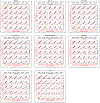
Extended Data Fig. 2. Evaluation of the composite likelihood model applied to extended nucleotide contexts.

To test the independence assumption of the composite likelihood model, we examined the interaction between any two positions (25 possible combinations) in the 11-nucleotide context around mutations of eight cancer types (bladder, n = 317 samples; breast, n = 1443; colorectal, n = 223; endometrium, n = 327; gastroesophageal, n = 833; head and neck, n = 425; lung adeno, n = 446; skin, n = 582). For any two positions, there are 96 possible nucleotide contexts and we plotted the observed mutation count of each nucleotide context (x-axis) against the predictions of the composite likelihood model (y-axis). Pearson correlation coefficients between observed and predicted data served as a measure of interaction. Each position pair is visualized in a separate correlation plot, and positions are annotated at the bottom right of the plot. For instance, pair (−1,1) refers to the trinucleotide context. Dot colors indicate the base substitution types.

Extended Data Fig. 3. Generalization of the composite likelihood model to extended nucleotide contexts.

We counted the number of mutations in each possible nucleotide context of length ≤7 based on the sequencing data of 11,873 samples. The exact number of samples per cancer type included in this analysis is shown in Extended Data Figure 5. We compared these counts with the mutability scores returned by the composite likelihood model (218,448 different nucleotide contexts). Since the number of possible nucleotide contexts was too large to be visualized directly, we plotted the data point density. The Pearson correlation coefficient (R) of each plot is annotated at the bottom right.

Extended Data Fig. 4. Extended nucleotide contexts contribute to the performance of the composite likelihood model.

We examined whether accounting for extended contexts beyond trinucleotide contexts improved the fit of the composite likelihood model. To this end, we varied the number of nucleotides in the composite likelihood model between 0 (i.e. only substitution types) and 6 (i.e. 7-nucleotide contexts). We computed the residual sum of squared differences between observed mutation counts and the predictions of the composite likelihood model. As a negative control, we determined the residual sum of squares for a uniform distribution. This baseline was used to normalize the residual sum of squares for each cancer type. For some cancer types with “flat” mutation signatures, nucleotide contexts only had minor impact on the fit of the model, but did not decrease the performance of the model (e.g., lung adeno., n = 446 samples). For other cancer types, the fit of the model largely depended on the trinucleotide context, but not on the extended nucleotide context (e.g., prostate cancer, n = 880). For most cancer types with high background mutation rates, the fit of the composite likelihood model strongly depended on the extended nucleotide context (e.g., bladder, n = 317; breast, n = 1443; cervical, n = 192; colorectal, n = 223; endometrial cancer, n = 327; melanoma, n = 582).

Extended Data Fig. 5. A large-scale cohort of whole-exome sequencing data to identify rare cancer genes.

To systematically identify candidate cancer genes, we analyzed sequencing data from 11,873 individual tumor samples using the statistical framework that we had developed in this study. Our study cohort contained whole-exome sequencing data from 32 TCGA-related (orange) and 55 TCGA-independent (blue) projects.

Extended Data Fig. 6. Benchmarking of the performance of MutPanning for cancer gene identification.

We benchmarked the performance of our method against 7 previously published methods for cancer gene identification based on the sequencing data of 11,873 samples spanning 28 different cancer types. The exact number of samples per cancer type can be found in Extended Data Figure 5. To benchmark the performance of a method, we sorted genes according to the significance values (adjusted for multiple testing) returned by the method. As a conservative approximation of the true-positive rate we used Cancer Gene Census (CGC) genes (a, b, c) and OncoKB genes (d, e, f) to derive ROC and precision-recall curves. We quantified the performance of each method as the area under the ROC curve (AUC) for the top 150 (a, d) or 1000 (b, e) non-CGC/OncoKB genes, respectively. Further, we determined the precision at 5% recall for each method (c, f). We normalized these measures to the maximum within each cancer type.

Extended Data Fig. 7. Comparison of different methods for cancer gene identification.

We benchmarked the performance of our method against 7 previously published methods for cancer gene identification based on the sequencing data of 11,873 samples spanning 28 different cancer types. To benchmark the performance of a method, we sorted genes according to the significance values (adjusted for multiple testing) returned by the method. As a conservative approximation of the true-positive rate we used Cancer Gene Census (CGC) genes (a, c, e) and OncoKB genes (b, d, f) to derive ROC and precision-recall curves. We quantified the performance of each method as the area under the ROC curve (AUC) for the top 150 (a, b) or 1000 (c, d) non-CGC/OncoKB genes, respectively. Further, we determined the precision at 5% recall for each method (e, f). Box plots indicate the distribution of these performance measures for each method across cancer types. Each cancer type is represented by a dot. Boxes indicate the 25%/75% interquartile range, whiskers extend to the 5%/95%-quantile range. The median of each distribution is indicated as a vertical line.

Extended Data Fig. 8. Comparison of performance measures derived from CGC vs. OncoKB.

We benchmarked the performance of our method against 7 previously published methods for cancer gene identification based on the sequencing data of 11,873 samples spanning 28 different cancer types. To benchmark the performance of a method, we sorted genes according to the significance values (adjusted for multiple testing) returned by the method. As a conservative approximation of the true-positive rate we used Cancer Gene Census (CGC) genes and OncoKB genes to derive ROC and precision-recall curves. We quantified the performance of each method as the area under the ROC curve (AUC) for the top 150 (a) or 1000 (b) non-CGC/OncoKB genes, respectively. Further, we determined the precision at 5% recall for each method (c). This figure compares the performance measures derived from the CGC (x-axis) and OncoKB (y-axis) databases. Each dot represents the AUC/precision of a different method (dot color) for an individual cancer type. The concordance between CGC and OncoKB measures suggests that our measure of performance does not entirely depend on the dataset used to approximate the true-positive rate.

Extended Data Fig. 9. Comparison of methods in two homogeneously processed datasets.

We compared the performance of MutPanning with 7 other methods on two independently processed datasets (TCGA subcohort (a-c, g-i), n = 7060 samples; MC3 dataset (d-f, j-l), n = 9079). We used the Cancer Gene Census (CGC) (a-f) and OncoKB (g-l) for benchmarking. We quantified the performance by the AUC of the ROC curve of the top 1,000 non-CGC/OncoKB genes returned by each method. a, d, g, j, Box plots indicate the distribution of performance measures for each method. Boxes indicate the 25%/75% interquartile range, whiskers extend to the 5%/95%-quantile range. Distribution medians are indicated as vertical lines. Each dot represents an AUC for one of the 27 cancer types in the TCGA and MC3 datasets. b, e, h, k, We normalized AUCs by the maximum AUC within each tumor type. We then compared these normalized AUCs between methods across cancer types. c, f, i, l, We compared the AUCs obtained from our original study cohort with the AUCs from TCGA and MC3 based on Pearson correlation. Each dot reflects a cancer type/method. Cohort sizes for TCGA/MC3 datasets: bladder: 130/386; blood: 197/139; brain: 576/821; breast: 975/779; cervix: 192/274; cholangio: 35/34; colorectal: 223/316; endometrium: 305/451; gastroesophageal: 467/529; head&neck: 279/502; kidney clear: 417/368; kidney non-clear: 227/340; liver: 194/354; lung adenocarcinoma: 230/431; lung squamous: 173/464; lymph: 48/37; ovarian: 316/408; pancreas: 149/155; pheochromocytoma: 179/179; pleura: 82/81; prostate: 323/477; sarcoma: 247/204; skin: 342/422; testicular: 149/145; thymus: 123/121; thyroid: 402/492; uveal melanoma: 80/80

Extended Data Fig. 10. Recurrent mutations in domains of protein-DNA interaction.

Significance values in this figure legend were computed using MutPanning and adjusted for multiple testing (false discovery rate, FDR). Recurrent SOX17 mutations in endometrial cancer (n = 327 samples, FDR = 8.77x10⁻³) are located in the high-mobility-group box domain at the SOX17-DNA interface (PDB: 4A3N superposed with 3F27). POLR2A harbors recurrent mutations in lung adenocarcinoma (n = 446, FDR = 9.28x10⁻⁶) at the end of an alpha helical segment that is directly pointed at the major groove of the double stranded DNA (PDB: 5IYB). The open complex of a cryo-EM multicomponent structure where the melted single-stranded template DNA is inserted into the active site and RNA polymerase II locates the transcription start site is visualized. CEBPA harbors recurrent mutations in hematological malignancies (n = 1018, FDR = 1.16x10⁻⁷) at the cross-over interface of the two CEBPA homodimers (PDB: 1NWQ). GATA3 (PDB: 4HCA) harbors recurrent mutations in breast cancer (n = 1443, FDR < 10⁻²⁰) at Asn334, which is located in the GATA-type 2 zinc finger (res317-res341), as well as the residue Met294, which is located peripheral to the GATA-type 1 zinc finger domain (res263-res287). RUNX1 harbors recurrent mutations in breast cancer (n = 1443, FDR = 2.22x10⁻⁴) and hematological malignancies (n = 1018, FDR = 1.94x10⁻⁵). Arg174 plays an important role for DNA recognition and facilitates the formation of hydrogen bond interactions to a guanosine base from the consensus DNA binding sequence of RUNX1 (PDB: 1H9D).

Fig. 1 ∣. Dependency of mutations on extended nucleotide contexts.

a, To identify driver genes, we searched for mutations in “unusual” nucleotide contexts that deviate from the context around passenger mutations. We combined this feature with other signals for driver gene identification. b, Bar graphs visualize how often each nucleotide occurs around recurrent mutations in bladder cancer (n = 317), endometrial cancer (n = 327) and melanoma (n = 582). c-d, We applied the composite likelihood model to the mutation frequency vectors of 9 COSMIC mutation signatures^-. For each trinucleotide context, we plotted the original frequency against the mutation frequency obtained from the composite likelihood model. e-f, We tested whether the composite likelihood model generalized to broader nucleotide contexts in 12 cancer types (bladder, n = 317; brain, n = 760; breast, n = 1443; cervix, n = 192; colorectal, n = 223; endometrial, n = 327; gastroesophageal, n = 833; head and neck, n = 425; lung adeno, n = 446; pancreas, n = 729; prostate, n = 880; skin, n = 582). For any three nucleotides in the 11-nucleotide context, we counted how many mutations were surrounded by the nucleotide triplet (n = 38,400 triplets, not necessarily adherent, ≥1 nucleotide on 5’ and 3’ sides). We plotted these counts against the prediction of the composite likelihood model. We compared original and modeled mutation frequencies by Pearson correlation coefficients (R). Plots for other mutation signatures and cancer types are provided in the supplement.

Fig. 2 ∣. Mutations in unusual contexts provide a signal in favor of driver genes.

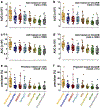
a, Based on 582 melanoma samples, we examined nucleotide contexts around mutations in 10 cancer and 5 non-cancer genes. We estimated the mutability of positions using the composite likelihood. We tested which positions contained more mutations than expected (one-sided test, binomial distribution) and adjusted for multiple testing (false discovery rate, FDR). We used an FDR threshold of 0.1 to classify whether the number of mutations per position was usual (gray) or unusual (orange) compared with its surrounding nucleotide context. Each nonsynonymous mutation is visualized as a dot. A small amount of jittering was added to separate mutations in the same position. b-c, Recurrence of mutations in the same position results from passenger mutations in highly mutable contexts or driver mutations in functionally important sites. Based on 582 melanoma samples, we examined whether nucleotide contexts could distinguish between these two possibilities. We gradually modulated the mutational likelihood cutoff (x-axis) from lowly mutable to highly mutable nucleotide contexts. For each cutoff, we computed the ratio of nonsynonymous to synonymous positions (b) and the fraction of positions in established cancer genes listed in the Cancer Gene Census^, (c). Error bars depict 95% confidence intervals based on the beta distribution, and dots indicate the distribution mean. As a negative control, we determined the same measures for positions without mutations. For sites with low mutational likelihood, recurrence is a better indicator of selection than for sites with high mutational likelihood.

Fig. 3 ∣. Comparison of different methods to identify driver genes.

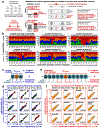
We benchmarked the performance of our method against seven other methods for driver gene identification. Since the full set of driver genes per cancer type is unknown, we used the Cancer Gene Census^, (CGC) for a conservative approximation of the true-positive rate (i.e. not every non-CGC gene is necessarily a false positive). Based on the top genes returned by each method, we plotted the number of non-CGC genes (x-axis) against the number of CGC genes (y-axis) until the list contained 1,000 non-CGC genes (inset: 150 non-CGC genes). This figure shows this benchmarking analysis for three cancer types with a high context dependency based on the TCGA subcohort (bladder, n = 130; endometrium, n = 305; skin, n = 342) and one cancer type with a low context dependency based on the TCGA subcohort (lung adeno., n = 230). Similar curves for other cancer types and the full study cohort are provided in Extended Data Figures 6-9 and the supplement.

Fig. 4 ∣. A catalog of driver genes in human cancer.

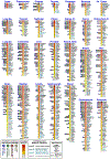
Based on whole-exome sequencing data from 11,873 tumor-normal pairs, we derived a catalog of driver genes across 28 cancer types. Extended Data Figure 5 lists the exact number of samples per cancer type. P-values were derived by our approach (MutPanning) and then adjusted for multiple testing. The most significant gene-tumor pairs (false discovery rate < 0.25) for each cancer type are listed in decreasing order of their mutation frequencies (color of the square next to the gene name, dark red to white). A maximum of 50 gene-tumor pairs is shown per cancer type. The full catalog can be found in Supplementary Table 3. The font size of the gene name reflects its significance. We compared our driver gene catalog to four catalogs from previous pan-cancer studies. Colored dots indicate which gene-tumor pairs were listed in previous catalogs. Font colors reflect which gene-tumor pairs had been reported in the literature (confidence levels A-D). Heterogeneity in variant calling, tissue collection protocols and mutation reports (synonymous mutations were not reported for 6.1% of the samples; studies marked in Supplementary Table 1) may represent a potential limitation for driver gene identification. We therefore ran MutPanning on two uniformly processed datasets (TCGA, n = 7,060 samples, and MC3, n = 9,079 samples) that did not have these limitations. We marked gene-tumor pairs that also reached statistical significance in this smaller dataset by asterisks (*). TCGA and MC3 datasets did not include adenoid cystic carcinoma.

Fig. 5 ∣. Stratification of driver genes based on literature support.

a, We stratified 827 gene-tumor pairs (based on 11,873 samples; significance values derived by MutPanning and adjusted for multiple testing) based on their literature support. Blue: gene-tumor pairs involving canonical cancer genes in the Cancer Gene Census (CGC)^,; orange/brown: genes-tumor pairs reported by experimental studies for the same/different tumor type as those identified by our method; gray: gene-tumor pairs with no literature support. b, Area-proportional Venn diagrams show the overlap in CGC genes between our catalog (orange) and catalogs from previous studies (green, red, blue, dark beige). The gray area reflects CGC gene-tumor pairs that were reported for the same tumor type in ≥2 independent catalogs. c, As a measure of consistency, we counted how many CGC genes from previous studies were also identified by our study (y-axis, fraction of CGC gene-tumor pairs in ≥2 independent catalogs). d, We counted the number of CGC gene-tumor pairs in our catalog that were not a part of previous studies. This measure reflects whether our catalog expanded existing catalogs by additional candidate driver genes. Our catalog (orange) recapitulated 85% of the CGC gene-tumor pairs from ≥2 previous studies (c), and contained 169 additional CGC gene-tumor pairs that were not a part of previous pan-cancer catalogs (d).

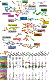
Fig. 6 ∣. Characterization of driver genes based on physical interactions.

a, Physical interactions between driver genes (based on 11,873 samples; identified by MutPanning) are visualized as a minimum-spanning tree based on a large-scale protein-protein interaction database. The color of each gene reflects its associated pathway, and the dot size indicates its maximum mutation frequency across the 28 cancer types examined in this study. b, We aggregated mutations across all driver genes in the same pathway and determined the relative contributions (dot sizes) of different pathways (rows) to the mutational landscape of 28 different cancer types (columns). The contribution of the most frequently mutated gene in each pathway is shown as a dark area within each dot.

References

1. Stratton MR, Campbell PJ & Futreal PA The cancer genome. Nature 458, 719–24 (2009). - PMC - PubMed
1. Vogelstein B et al. Cancer genome landscapes. Science 339, 1546–58 (2013). - PMC - PubMed
1. Stephens PJ et al. The landscape of cancer genes and mutational processes in breast cancer. Nature 486, 400–4 (2012). - PMC - PubMed
1. Greaves M & Maley CC Clonal evolution in cancer. Nature 481, 306–13 (2012). - PMC - PubMed
1. Bailey MH et al. Comprehensive Characterization of Cancer Driver Genes and Mutations. Cell 173, 371–385 e18 (2018). - PMC - PubMed
References (Online Methods)
1. Gao J et al. Integrative analysis of complex cancer genomics and clinical profiles using the cBioPortal. Sci Signal 6, pl1 (2013). - PMC - PubMed
1. Cerami E et al. The cBio cancer genomics portal: an open platform for exploring multidimensional cancer genomics data. Cancer Discov 2, 401–4 (2012). - PMC - PubMed
1. Lek M et al. Analysis of protein-coding genetic variation in 60,706 humans. Nature 536, 285–91 (2016). - PMC - PubMed
1. Costello M et al. Discovery and characterization of artifactual mutations in deep coverage targeted capture sequencing data due to oxidative DNA damage during sample preparation. Nucleic Acids Res 41, e67 (2013). - PMC - PubMed
1. Gilson MK et al. BindingDB in 2015: A public database for medicinal chemistry, computational chemistry and systems pharmacology. Nucleic Acids Res 44, D1045–53 (2016). - PMC - PubMed
Publication types