The Modern-Era Retrospective Analysis for Research and Applications, Version 2 (MERRA-2)

Abstract

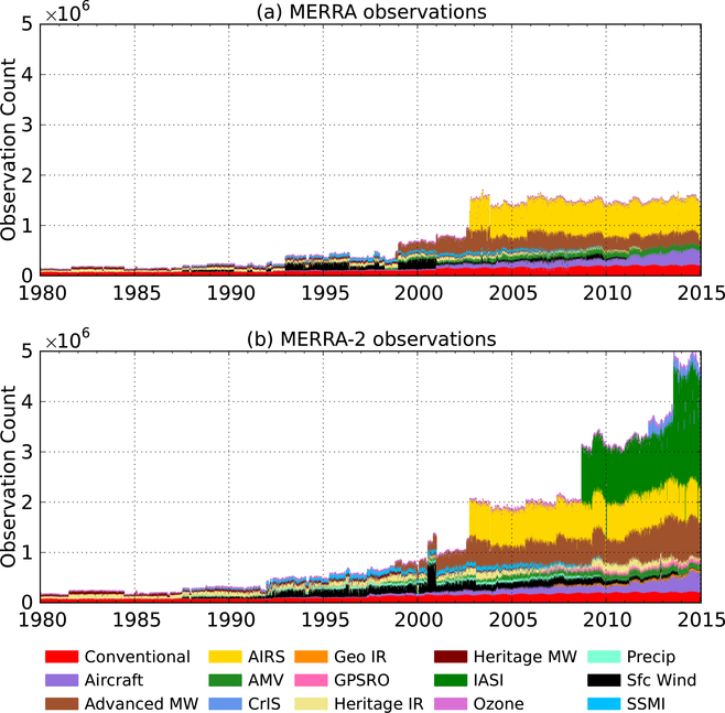
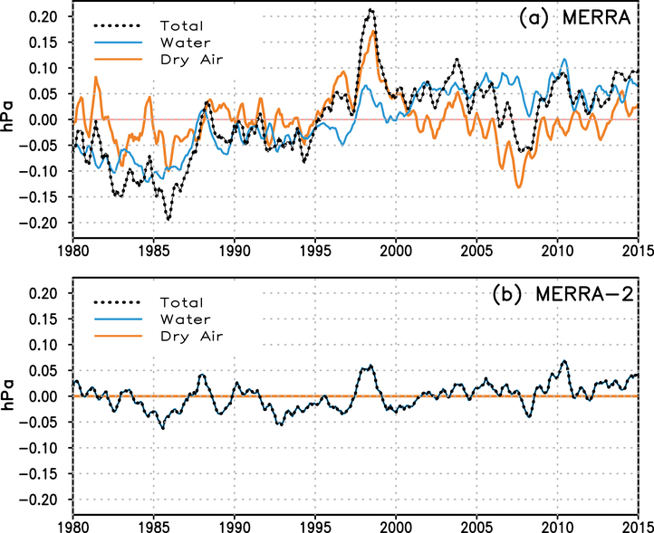
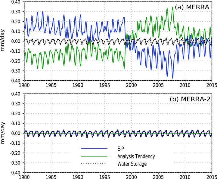
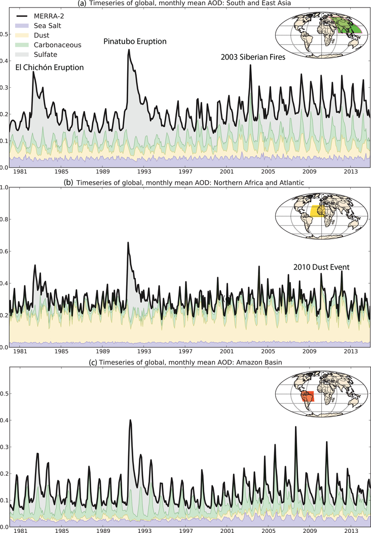
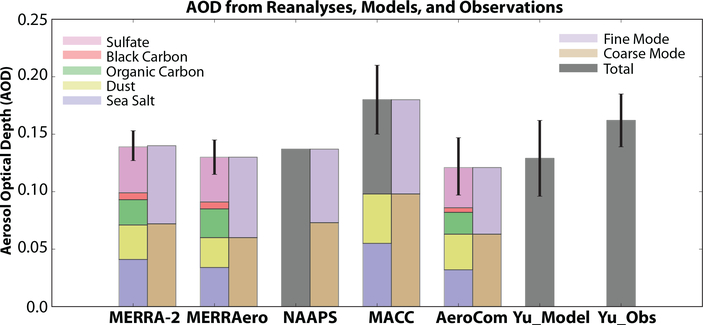
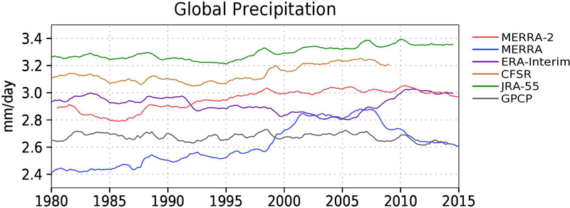
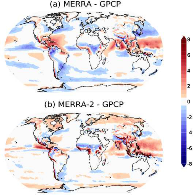
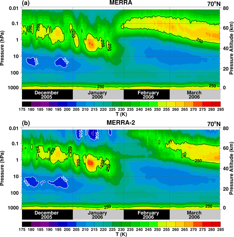
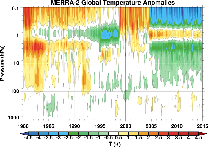
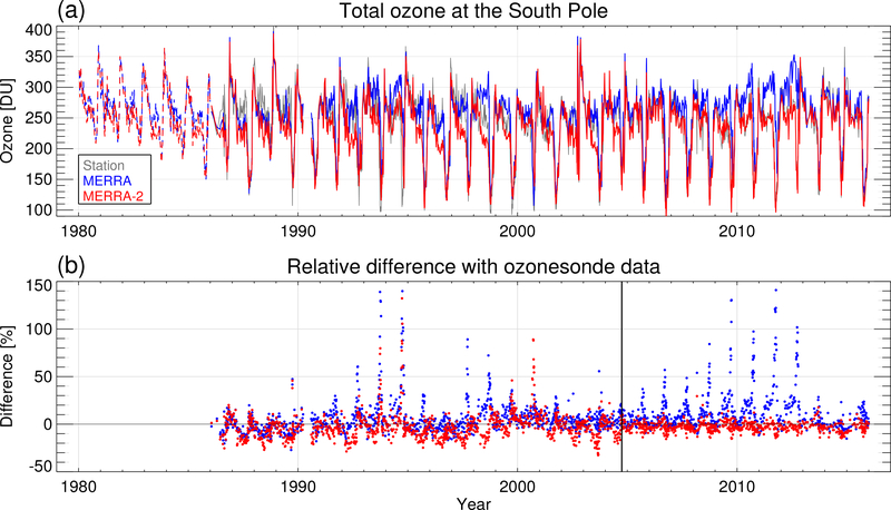
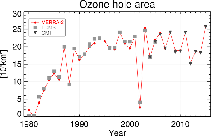
The Modern-Era Retrospective Analysis for Research and Applications, Version 2 (MERRA-2) is the latest atmospheric reanalysis of the modern satellite era produced by NASA's Global Modeling and Assimilation Office (GMAO). MERRA-2 assimilates observation types not available to its predecessor, MERRA, and includes updates to the Goddard Earth Observing System (GEOS) model and analysis scheme so as to provide a viable ongoing climate analysis beyond MERRA's terminus. While addressing known limitations of MERRA, MERRA-2 is also intended to be a development milestone for a future integrated Earth system analysis (IESA) currently under development at GMAO. This paper provides an overview of the MERRA-2 system and various performance metrics. Among the advances in MERRA-2 relevant to IESA are the assimilation of aerosol observations, several improvements to the representation of the stratosphere including ozone, and improved representations of cryospheric processes. Other improvements in the quality of MERRA-2 compared with MERRA include the reduction of some spurious trends and jumps related to changes in the observing system, and reduced biases and imbalances in aspects of the water cycle. Remaining deficiencies are also identified. Production of MERRA-2 began in June 2014 in four processing streams, and converged to a single near-real time stream in mid 2015. MERRA-2 products are accessible online through the NASA Goddard Earth Sciences Data Information Services Center (GES DISC).

Figure 1:

Observations assimilated per 6-hr cycle in (a) MERRA and (b) MERRA-2. The temporary spike in the number of surface wind observations assimilated in MERRA-2 in late 2000 is due to an error in the pre-processing of QuikSCAT data.

Figure 2:

Globally integrated monthly-mean mass anomalies from the mean seasonal cycle for (a) MERRA and (b) MERRA-2. Shown are the anomalies of total mass (black dotted), and their decomposition into atmospheric water (blue) and dry air (orange). The units are hPa. Results for MERRA-2 are derived from the data collection described in GMAO (2015b).

Figure 3:

Globally integrated monthly-mean total water budget terms for (a) MERRA and (b) MERRA-2. Shown are the water source term (E − P, blue), vertically integrated analysis increment of water (green), and atmospheric water storage (black dotted). The units are mm day⁻¹. Results for MERRA-2 are derived from the data collections described in GMAO (2015b, d, e).

Figure 4:

Mean difference (1980–2015) between the (corrected) MERRA-2 precipitation seen by the land surface and the model-generated precipitation within the MERRA-2 system. The units are mm d⁻¹. Results are derived from the data collections described in GMAO (2015h, j).

Figure 5:

Time series of 12-month running mean prescribed sea surface temperature for various reanalyses, averaged between 60°N and 60°S. The units are K. Results for MERRA-2 are derived from the data collection described in GMAO (2015f).

Figure 6:

Monthly mean (thick lines) and RMS (thin lines) background departures for surface pressure observations assimilated in MERRA (blue) and MERRA-2 (red). Results are shown for the (a) Northern Hemisphere and (b) Southern Hemisphere. The units are hPa. Also shown are the corresponding monthly mean counts of surface pressure observations assimilated in MERRA-2 (gray shaded).

Figure 7:

Global monthly mean (thick lines) and RMS (thin lines) background departures for radiosonde temperature observations assimilated in MERRA (blue) and MERRA-2 (red). Results are shown for the pressure levels (a) 10 hPa, (b) 50 hPa, (c) 300 hPa and (d) 700 hPa. The units are K. Also shown are the corresponding monthly mean counts of radiosonde temperature observations assimilated in MERRA-2 (gray shaded).

Figure 8:

As in Figure 7, except for radiosonde specific humidity observations in the tropics (20°N-20°S) at (a) 500 hPa and (b) 850 hPa. The units are g kg⁻¹.

Figure 9:

(a) Mean and (b) standard deviation of the monthly mean analysis tendency of surface pressure for the period January 1980 through December 2015. Monthly mean values are based on four synoptic times daily. The units are hPa day⁻¹. Results are derived from the data collection described in GMAO (2015k).

Figure 10:

Global (a) mean and (b) standard deviation of the monthly mean analysis tendency of temperature from 1000 to 70 hPa. Monthly means values are based on four synoptic times daily. The units are K day⁻¹. Results are derived from the data collection described in GMAO (2015n).

Figure 11:

As in Figure 10, except for specific humidity in the tropics (20°N-20°S) from 1000 to 250 hPa. The units are g kg⁻¹ day⁻¹. Results are derived from the data collection described in GMAO (2015l).

Figure 12:

Probability distribution functions (PDFs) of observation minus forecast (O-F, dashed) and observation minus analysis (O-A, solid) differences in observation space, collocated in space and time for each sensor in the MERRA-2 aerosol observing system. The PDFs are calculated from innovation data in log-transformed space (ln(AOD+0.01)) to ensure distributions are positive and Gaussian. The time periods considered include AVHRR (1993–1999), MODIS Terra (2001–2014), MODIS Aqua (2003–2014), MISR (2001–2012), and AERONET (ANET 2000–2013).

Figure 13:

Time series of area-weighted aerosol optical depth (AOD) from the MERRA-2 aerosol reanalysis averaged over major aerosol source regions: (a) South and East Asia [5°N-55°N, 65°W-160°W], (b) northern Africa [2.5°S-30°N, 45°W-15°E], and (c) the Amazon Basin in South America [20°S-7.5°N, 80°W-30°W]. The total AOD (thick black line) is the sum of contributions from sea salt (blue), dust (yellow), carbonaceous (black and organic carbon, green), and sulfate (grey) AOD. Results are derived from the data collection described in GMAO (2015g).

Figure 14:

Aerosol optical depth (AOD) from aerosol reanalyses (MERRA-2, MERRAero, NAAPS, MACC), inter-model comparisons (AeroCom Phase I, Yu_Model), and observations (Yu_Obs) for the period 2003–2010. Where available, total AOD is broken down by component species (left bar) and by fine and coarse mode (right bar). For MERRA-2 and MERRAero, the error bar represents the standard deviation of the monthly-mean AOD for the period 2003–2010. For MACC, the error bar is the uncertainty in the total AOD from Bellouin et al. (2013). AeroCom (Kinne et al., 2006) and Yu et al. (2006) uncertainty are the inter-model or inter-observational standard deviations. Coarse mode is defined as the sum of dust plus sea salt AOD, with the remainder of the AOD assigned to the fine mode. Results for MERRA-2 are derived from the data collection described in GMAO (2015g).

Figure 15:

Time series of 12-month running mean globally averaged precipitation for several reanalyses and the GPCP merged gauge satellite data product. The units are mm day⁻¹. Results for MERRA-2 are derived from the data collection described in GMAO (2015h).

Figure 16:

Time-averaged precipitation differences during June-July-August for (a) MERRA minus GPCP and (b) MERRA-2 minus GPCP for the period 1980–2015. The units are mm day⁻¹. Results for MERRA-2 are derived from the data collection described in GMAO (2015h).

Figure 17:

Time series of midwestern US summer seasonal precipitation anomalies, following Bosilovich (2013). The anomalies are computed from the June-July-August mean for the period 1980–2011. The gauge data are from NOAA/CPC gridded daily data for the US (Xie et al. 2007). The units are mm day⁻¹. Results for MERRA-2 are derived from the data collection described in GMAO (2015h).

Figure 18:

Regional summary statistics for the US summer seasonal anomaly time series of precipitation: (a) mean (mm day⁻¹), (b) standard deviation (mm day⁻¹ ), and (c) anomaly correlation to CPC gauge observations. The anomalies are computed from the June-July-August mean for the period 1980–2011. The regions lie within the continental US and are defined as in Bosilovich (2013): Northeast (NE), Southeast (SE), Midwest (MW), Great Plains (GP), Southern Great Plains (SGP), Northern Great Plains (NGP), Northwest (NW), Southwest (SW), and the accumulation of all area in these regions (US). Results for MERRA-2 are derived from the data collection described in GMAO (2015h).

Figure 19:

Average amount of precipitation that exceeds the 99th percentile during June-July-August for the period 1980–2013 for (a) MERRA, (b) MERRA-2, and (c) CPC gauge observations. Panel (d) shows the closeness of each reanalysis to the CPC observations for the same period, defined as |MERRA-2 − CPC| − |MERRA − CPC|, where the vertical bars indicate absolute differences and the names indicate the set of time-averaged grid-point values for each data type. In (d), blue (red) shades indicate that MERRA-2 (MERRA) is closer to the CPC observations. The units in all panels are mm day⁻¹. Results for MERRA-2 are derived from the data collection described in GMAO (2015d).

Figure 20:

Ertel’s potential vorticiity (EPV, ×10³ potential vorticity units, PVU; 1 PVU = 10⁻⁶m⁻²s⁻¹K kg⁻¹) at 0.7 hPa on 2 January 1995 12 UTC for (a) MERRA and (b) MERRA-2 for the Northern Hemisphere. Polar cap detail (80°−90°N) for (c) MERRA and (d) MERRA-2. Color shading interval is 2.5 × 10³ PVU. Black contour interval is 10 × 10³ PVU in (a) and (b) and 5 × 10³ PVU in (c) and (d). Cyan circle denotes 80°N latitude. Results are derived from the data collection described in GMAO (2015c).

Figure 21:

Time-altitude section of zonally averaged temperature at 70°N for (a) MERRA and (b) MERRA-2. The time resolution is twice daily (00 and 12 UTC) for December 2005-March 2006. The contour interval is 5 K.

Figure 22:

Monthly and globally averaged temperature anomaly for MERRA-2 as a function of time. The annual cycle and mean for 1980–2015 have been removed. The MLS temperatures were introduced at levels above 5 hPa beginning in August 2004. Results are derived from the data collection described in GMAO (2015c).

Figure 23:

Time series of (a) total ozone (Dobson units, DU) at the South Pole derived from individual ozonesonde measurements (gray) and from collocated values in MERRA (blue) and MERRA-2 (red). Note that ozonesonde measurements are unavailable prior to 1986; see text for details. The reanalysis-minus-ozonesonde differences divided by sonde total ozone are shown in (b) for MERRA (blue) and MERRA-2 (red). The black vertical line in (b) separates the SBUV and Aura periods. (Figure from Wargan et al. 2016.) Results for MERRA-2 are derived from the data collection described in GMAO (2015a).

Figure 24:

Time series of the Antarctic ozone hole area calculated from MERRA-2 ozone fields averaged between 20 September and 10 October for the years 1980–2015 (red curve with circles). Also shown are values derived from TOMS (gray squares) and OMI (black triangles) observations. The units are 10⁶ km². Results for MERRA-2 in 1994 are excluded due to insufficient SBUV data coverage in the Southern Hemisphere, which significantly degraded the analysis; see text for details. Results for MERRA-2 are derived from the data collection described in GMAO (2015a).

Figure 25:

Average annual cycle of 2-m air temperature in MERRA and MERRA-2 at (a) South Pole station (90°S; 1980–2014; Turner et al., 2004), (b) Gill automatic weather station (80°S, 179°W; 1985–2014; Turner et al., 2004), and (c) Summit, Greenland (73°N, 38°W; 2000–2002; Hoch, 2005). The units are °C. Vertical bars denote ±1 standard deviation of the multi-year time series for each month. Results for MERRA-2 are derived from the data collections described in GMAO (2015i, j, m).

Figure 26:

Surface mass balance for the Greenland Ice Sheet for the period 1980–2012 in (a) MERRA, (b) MERRA-2, and (c) MAR regional climate model (Fettweis 2007). The units are mm yr⁻¹ water-equivalent. Surface topography (including ice sheet) is contoured with dashed lines every 200 m. Results for MERRA-2 are derived from the data collections described in GMAO (2015i, j, m).

References

1. Adler RF, and Coauthors, 2003: The version-2 Global Precipitation Cimatology Project (GPCP) monthly precipitation analysis (1979-present). J. Hydrometeor, 4, 1147–1167. - PMC - PubMed
1. Akella S, Todling R, M., and Suárez M, 2016: Assimilation for skin SST in the NASA GEOS atmospheric data assimilation system. Quart. J. Roy. Meteor. Soc, doi:10.1002/qj.2988. - DOI - PMC - PubMed
1. Andrews DG, Holton JR, and Leovy CB, 1987: Middle Atmosphere Dynamics. Academic Press, 489 pages.
1. Bacmeister JT and Stephens G, 2011: Spatial statistics of likely convective clouds in CloudSat data. J. Geophys. Res, 116, D04104, doi:10.1029/2010JD014444. - DOI
1. Ballish BA, and Kumar VK, 2008: Systematic differences in aircraft and radiosonde temperatures. Bull. Amer. Meteor. Soc, 89, 1689–1707.
LinkOut - more resources