Artificial Intelligence for MR Image Reconstruction: An Overview for Clinicians

Abstract

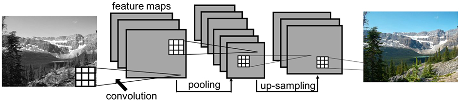
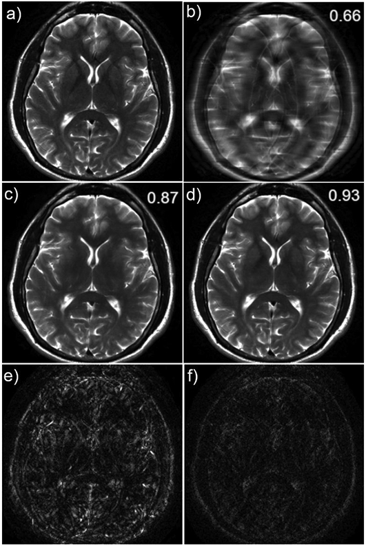
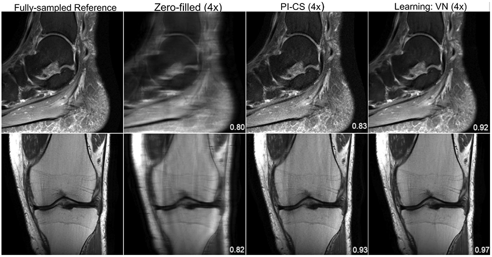
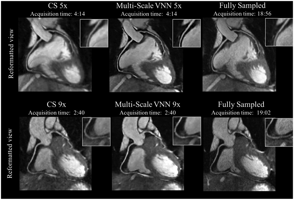
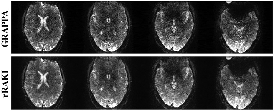
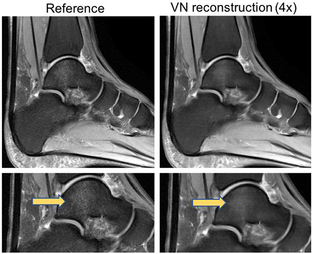
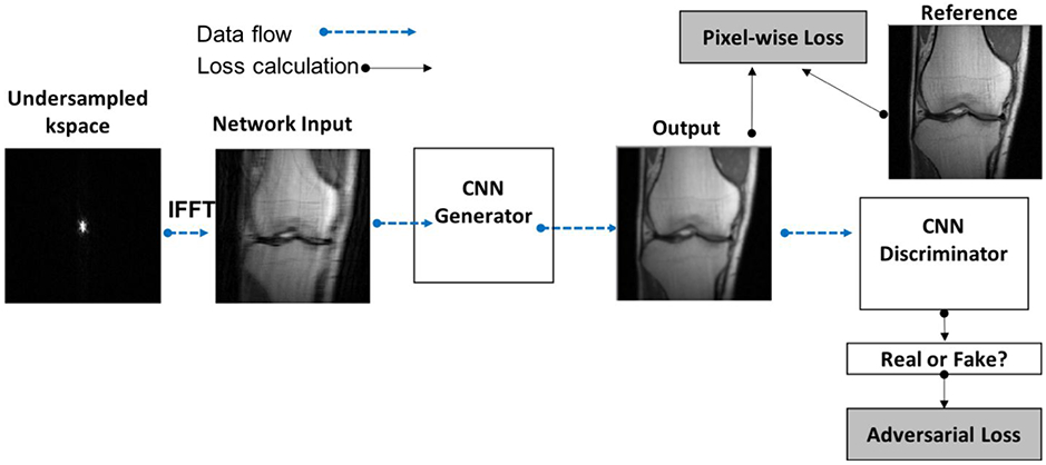
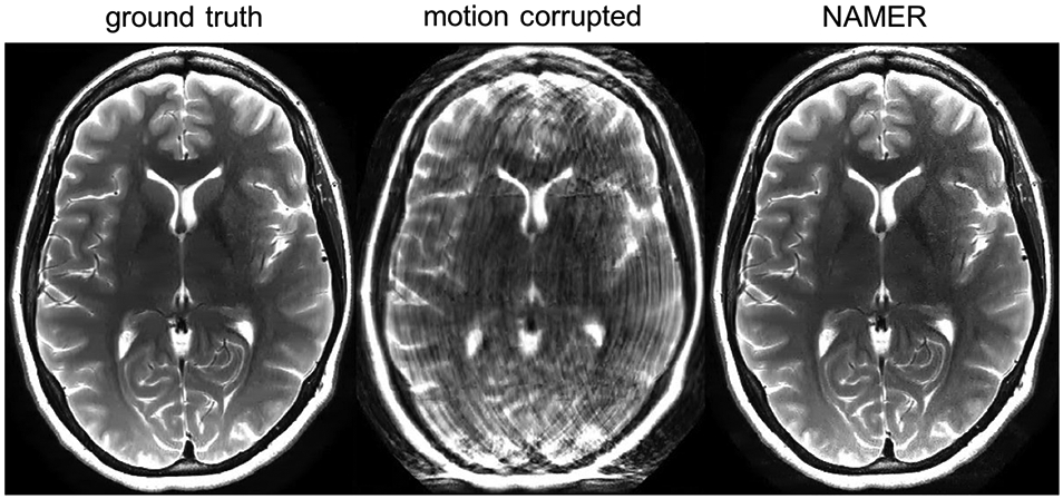
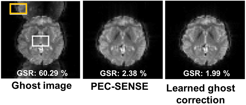
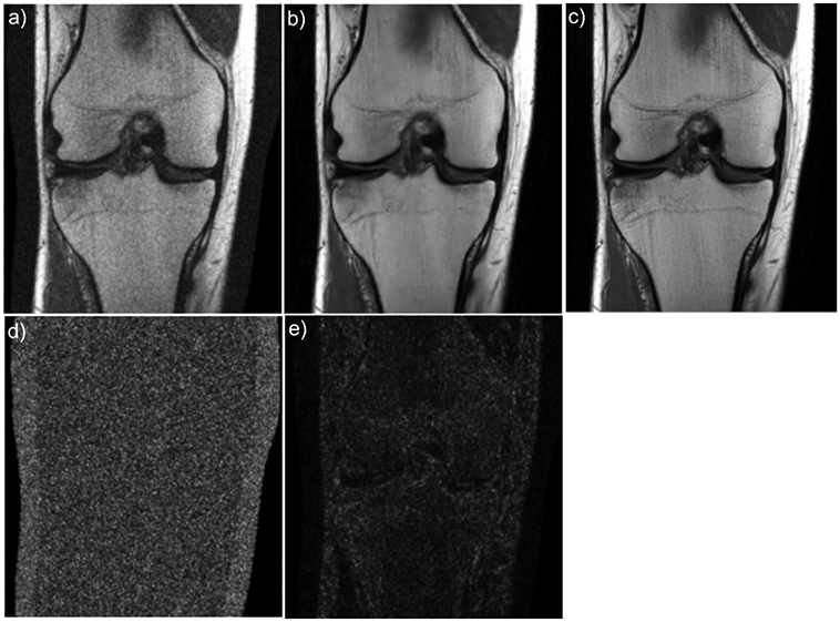
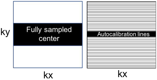
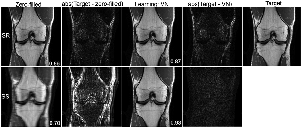
Artificial intelligence (AI) shows tremendous promise in the field of medical imaging, with recent breakthroughs applying deep-learning models for data acquisition, classification problems, segmentation, image synthesis, and image reconstruction. With an eye towards clinical applications, we summarize the active field of deep-learning-based MR image reconstruction. We review the basic concepts of how deep-learning algorithms aid in the transformation of raw k-space data to image data, and specifically examine accelerated imaging and artifact suppression. Recent efforts in these areas show that deep-learning-based algorithms can match and, in some cases, eclipse conventional reconstruction methods in terms of image quality and computational efficiency across a host of clinical imaging applications, including musculoskeletal, abdominal, cardiac, and brain imaging. This article is an introductory overview aimed at clinical radiologists with no experience in deep-learning-based MR image reconstruction and should enable them to understand the basic concepts and current clinical applications of this rapidly growing area of research across multiple organ systems.

Keywords: MRI; deep learning; image reconstruction.

Figure 1.

Example of a convolutional neural network (CNN) to predict image colors. The CNN takes the input image and estimates the red, green, blue components of the image, based on learned features extracted from the image by the convolution kernels. The square grids represent convolution kernels, which are made up of trainable weights. Each voxel in a feature map is the result of a convolution operation applied to the previous layer (illustrated by the connecting lines). An image processing CNN typically will have an encoder-decoder style architecture, which contains pooling layers followed by upsampling layers. In this didactic example, the network has 4 convolutional layers as well as a pooling layer (encoding) and an up-sampling layer (decoding). The CNN ultimately learns to synthesize a color image from a black and white image given many training pairs.

Figure 2.

Example illustrating the difference between image post-processing and image reconstruction of a 4X accelerated T2-weighted brain image. These results were obtained using a convolutional neural network for image reconstruction (4) and a modified version of this network not utilizing the raw data for image post-processing. The fully-sampled reference is shown in (a), and the zero-filled reconstruction in (b). The image post-processing result is shown in (c) and the reconstruction result is shown in (d). The absolute errors are shown in (e) and (f). The displayed values are structural similarity index (SSIM) (60) – a measure of similarity between the network output and the target, in this case the fully-sampled image (a). SSIM values range from 0 to 1, where 1 indicates perfect agreement. In this example of generating high-quality images from under-sampled data, the result obtained from the image reconstruction tool utilizes information from the raw data and outperforms the post-processing tool. The reconstruction has fewer residual artifacts and less blurring with better preservation of important structures such as the globus pallidus. It has not been established in the literature whether image reconstruction will always outperform image post-processing, or vice versa, in other applications.

Figure 3.

From left to right: A single slice of the reference, zero-filled, PI-CS and VN reconstructions of a sagittal, proton-density weighted, fat-suppressed ankle image (top) and a coronal proton-density weighted knee image (bottom). The displayed structural similarity index (SSIM) was calculated for the presented slice. The VN reconstruction has less noise amplification and residual artifact than the PI-CS reconstruction. The sequence parameters were as follows: ankle – sagittal fat-saturated proton-density (PD-FS): TR = 2800 ms, TE = 30 ms, turbo factor (TF) = 5, matrix size = 384 x 384, in-plane resolution 0.42 x 0.42 mm², slice thickness = 3.0 mm; knee – coronal PD: TR = 2750 ms, TE = 32 ms, TF = 4, matrix size = 320 x 320, in-plane resolution = 0.44 x 0.44 mm², slice thickness = 3.0 mm.

Figure 4.

Coronary MR angiography (CMRA) images reformatted along the left anterior descending and right coronary arteries for two representative healthy subjects. Acquisitions were performed with isotropic resolution 1.2 mm³ and 100% respiratory scan efficiency (no respiratory gating). Prospective undersampled acquisitions with acceleration factors 5x (first row) and 9x (second row) are shown. Images were reconstructed using a Wavelet-based compressed-sensing reconstruction (CS) and a Multi-Scale variational neural network (MS-VNN) reconstruction framework. Corresponding (consecutively acquired) fully-sampled acquisitions are shown in the last column for comparison. MS-VNN provides higher image quality than CS for both acceleration factors, achieving similar image quality to the fully-sampled reference. The reconstruction of a whole 3D CMRA volume took ~14s with MS-VNN. In comparison, the reconstruction for Wavelet-based CS was 5 minutes on average. Figure courtesy of Claudia Prieto.

Figure 5.

GRAPPA (top) and RAKI (bottom) reconstruction of simultaneous multi-slice (SMS) echo planar images (EPI) of the brain. SMS imaging acquires multiple slices at the same time (16 in this example) and is traditionally reconstructed with GRAPPA. RAKI reconstruction of SMS-EPI brain images outperforms GRAPPA reconstruction with decreased noise (61). Figure courtesy of Mehmet Akcakaya.

Figure 6.

Example of oversmoothing from deep learning reconstruction. Sagittal fat-saturated proton-density weighted images of the ankle of the fully sampled reference (left column) and the VN reconstruction (right column) demonstrate the oversmoothed appearance that can occur with these deep learning reconstruction methods, rendering such images easily distinguishable from those reconstructed conventionally. Note the loss of detail of the normal trabecular architecture that is present generally across the entire image and the decreased conspicuity of the focal talar dome bone marrow edema (arrows) on the VN reconstructed image (bottom right). The bottom images are cropped and magnified from corresponding images in the top row.

Figure 7.

Flow chart illustrating a generative adversarial network (GAN). Every GAN is made up of two CNNs, a generator and a discriminator. Incorporating the adversarial loss forces the generator to produce images that are indistinguishable from target images. The methods described in Mardani et al, Quan et al and Yang et al all have this general architecture; the main difference between methods lies in how data consistency is enforced.

Figure 8.

NAMER motion correction of a 2D T2-weighted brain image. Figure courtesy of Melissa Haskell.

Figure 9.

Ghost correction results of 3T GRE-EPI in vivo data demonstrating improved image quality defined as ghost-to-signal ratio (GSR), when comparing the learned ghost correction and phase error correction with sensitivity encoding (PEC-SENSE), a conventional method of ghost artifact correction. The lower the GSR value, the better the image quality. Example ROIs for ghost and signal values are depicted by the orange and white rectangles, respectively. Figure courtesy of Jong Ye.

Figure 10.

Example VN image denoising result. In these experiments Gaussian noise was added to coronal proton density weighted knee images and the noisy/clean image pairs were used to train the VN. The network was trained using the Adam optimizer with a learning rate of 1x10-3 and a batch size of 1 for 20 epochs. A coronal proton-density weighted image of the knee with added noise (a), the network output (b), and the target image (c). The absolute value of the difference between the target and noisy images and between the target and network output are shown in (d) and (e), respectively.

Figure 11.

Illustration of k-space sampling patterns for super-resolution (left) and sparse sampling (right). The black regions and lines represent acquired k space lines. The white regions are zero-filled.

Figure 12.

Reconstruction results of a 3x accelerated coronal proton-density weighted knee image for super resolution (SR) and sparse sampling (SS). The displayed structural similarity index (SSIM) values and difference images are provided for the presented slice. The variational network, implemented in Pytorch, was trained on 20 proton density weighted coronal knee images with the two sampling patterns illustrated in Figure 11. The network was trained using the Adam optimizer with a learning rate of 1x10-3 and a batch size of 1 for 30 epochs. One of the undersampling patterns is consistent with an acceleration factor of 4, where 24 center lines were acquired along with every 4th line outside the center region. The other undersampling pattern had the same number of acquired lines, restricted entirely to the center of k space. An alternative to regularly spaced undersampling is non-uniform undersampling, typically used with compressed sensing applications. Previous work has shown that uniform and non-uniform undersampling perform comparably for deep learning reconstructions (28,54).

References

1. Chan HP, Doi K, Galhotra S, Vyborny CJ, MacMahon H, Jokich PM. Image feature analysis and computer-aided diagnosis in digital radiography. I. Automated detection of microcalcifications in mammography. Med Phys 1987;14(4):538–548. - PubMed
1. MacMahon H, Doi K, Chan HP, Giger ML, Katsuragawa S, Nakamori N. Computer-aided diagnosis in chest radiology. J Thorac Imaging 1990;5(1):67–76. - PubMed
1. Castellino RA. Computer aided detection (CAD): an overview. Cancer Imaging 2005;5:17–19. - PMC - PubMed
1. Hosny A, Parmar C, Quackenbush J, Schwartz LH, Aerts H. Artificial intelligence in radiology. Nat Rev Cancer 2018;18(8):500–510. - PMC - PubMed
1. McBee MP, Awan OA, Colucci AT, et al. Deep Learning in Radiology. Acad Radiol 2018;25(11):1472–1480. - PubMed
Publication types