Overtone focusing in biphonic tuvan throat singing

Abstract

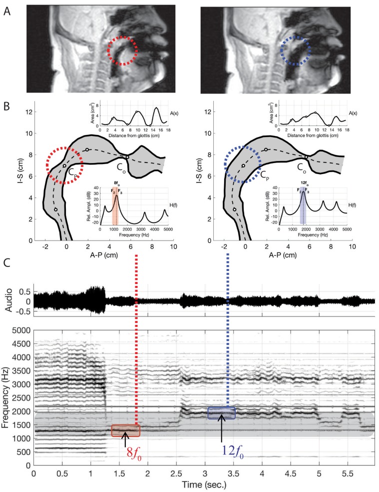
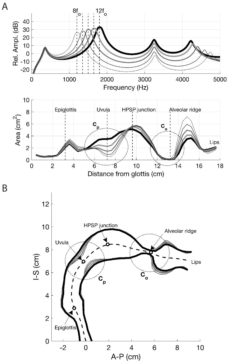
Khoomei is a unique singing style originating from the republic of Tuva in central Asia. Singers produce two pitches simultaneously: a booming low-frequency rumble alongside a hovering high-pitched whistle-like tone. The biomechanics of this biphonation are not well-understood. Here, we use sound analysis, dynamic magnetic resonance imaging, and vocal tract modeling to demonstrate how biphonation is achieved by modulating vocal tract morphology. Tuvan singers show remarkable control in shaping their vocal tract to narrowly focus the harmonics (or overtones) emanating from their vocal cords. The biphonic sound is a combination of the fundamental pitch and a focused filter state, which is at the higher pitch (1-2 kHz) and formed by merging two formants, thereby greatly enhancing sound-production in a very narrow frequency range. Most importantly, we demonstrate that this biphonation is a phenomenon arising from linear filtering rather than from a nonlinear source.

Keywords: Tuvan throat singing; acoustic phonetics; biphonation; human; physics of living systems; speech biomechanics.

Figure 1.. Frequency spectra for three different singers transitioning from normal to biphonic singing.

Vertical white lines in the spectrograms (left column) indicate the time point for the associated spectrum in the right column. Transition points from normal to biphonic singing state are denoted by the red triangle. The fundamental frequency ($f_0$) of the song is indicated by a peak in the spectrum marked by a green square. Overtones, which represent integral multiples of this frequency, are also indicated (black circles). Estimates of the formant structure are shown by overlaying a red dashed line and each formant peak is marked by an x. Note that the vertical scale is in decibels (e.g., a 120 dB difference is a million-fold difference in pressure amplitude). See also Appendix 1—figure 1 and Appendix 1—figure 2 for further quantification of these waveforms. The associated waveforms can be accessed in the Appendix [T1_3short.wav, T2_5short.wav, T3_2shortA.wav].

Figure 2.. A waterfall plot representing the spectra at different time points as singer T2 transitions from normal singing into biphonation (T2_3short.wav).

The superimposed arrows are color-coded to help visualize how the formants change about the transition, chiefly with F3 shifting to merge with F2. This plot also indicates the second focused state centered just above 3 kHz is a sharpened F4 formant.

Figure 3.. 3-D reconstruction of volumetric MRI data taken from singer T2 (Run3; see Appendix, including Appendix 1—figure 18).

(A) Example of MRI data sliced through three different planes, including a pseudo-3D plot. Airspaces were determined manually (green areas behind tongue tip, red for beyond). Basic labels are included: L – lips, J – jaw, To– tongue, AR – alveolar ridge, V – velum, E – epiglottis, Lx – larynx, and Tr – trachea. The shadow from the dental post is visible in the axial view on the left hand side and stops near the midline leaving that view relatively unaffected. (B) Reconstructed airspace of the vocal tract from four different perspectives. The red circle highlights the presence of the piriform sinuses (Dang and Honda, 1997).

Figure 4.. Analysis of vocal tract configuration during singing.

(A) 2D measurement of tract shape. The inner and outer profiles were manually traced, whereas the centerline (white dots) was found with an iterative bisection technique. The distance from the inner to outer profile was measured along a line perpendicular to each point on the centerline (thin white lines). (B) Collection of cross-distance measurements plotted as a function of distance from the glottis. Area function can be computed directly from these values and is derived by assuming the cross-distances to be equivalent diameters of circular cross-sections (see Materials and methods). (C) Schematic indicating associated modeling assumptions, including vocal tract configuration as in panel B (adapted from Bunton et al. (2013), under a Creative Commons CC-BY license, https://creativecommons.org/licenses/by/4.0/). (D) Model frequency response calculated from the associated area function stemming from panels B and C. Each labeled peak can be considered a formant frequency and the dashed circle indicates merging of formants F2 and F3.

Figure 5.. Results of changing vocal tract morphology in the model by perturbing the baseline area function A0⁢(x) to demonstrate the merging of formants F2 and F3, atop two separate overtones as apparent in the two columns of panels A and B.

(A) The frames from dynamic MRI with red and blue dashed circles highlighting the location of the key vocal tract constrictions. (B) Model-based vocal tract shapes stemming from the MRI data, including both the associated area functions (top inset) and frequency response functions (bottom inset). $C_O$ indicates the constriction near the alveolar ridge while $C_P$ the constriction near the uvula in the upper pharynx. (C) Waveform and corresponding spectrogram of audio from singer T2 (a spectrogram from the model is shown in Appendix 1—figure 14). Note that the merged formants lie atop either the 7th overtone (i.e., $8f_0$) or the 11th (i.e., $12f_0$).

Appendix 1—figure 1.. Same as Figure 1 (middle left panel; subject T2, same sound file as shown in the middle panel of Figure 1), except with overtones and estimated formant structure tracked across time.

Appendix 1—figure 2.. Same data/layout as in Figure 1 but now showing eR⁢(1,2) as defined in the 'Materials and methods'.

These plots show the energy ratio focused between 1–2 kHz. Vertical red dashed lines indicate approximate time of transition into the focused state. An expanded timescale is also shown for singer T2 (middle panel) in Appendix 1—figure 3.

Appendix 1—figure 3.. Similar to Figure 2 for singer T2 (middle panel), except an expanded time scale is shown to demonstrate the earlier dynamics as this singer approaches the focused state (see T2_5longer.wav).

Appendix 1—figure 4.. Stemming directly from Figure 1, the right-hand column now shows a spectrum from a time point prior to transition into the focused state (as denoted by the vertical black lines in the left column).

The shape of the spectra from Figure 1 is also included for reference.

Appendix 1—figure 5.. Spectrogram for singer T4 singing in non-Sygyt style (first song segment of T2_4shortA.wav sound file).

For the spectrogram, 4096 point windows were used for the fast Fourier transform (FFT) with 95% fractional overlap and a Hamming window.

Appendix 1—figure 6.. Spectrogram of the entire T2_5.wav sound file.

The sample rate was 96 kHz. The analysis parameters used were the same as those used for Figure 5.

Appendix 1—figure 7.. Spectrogram of the first song segment of the T1_3.wav sound file.

The analysis parameters used were the same as those for Figure 5.

Appendix 1—figure 8.. Singer T2's transition into a focused state.

Note that while the first focused state transitions from approximately 1.36 to 1.78 kHz, the second state remains nearly constant, decreasing only slightly from 3.32 to 3.17 kHz (T2_1shortB.wav).

Appendix 1—figure 9.. Spectrogram of singer T2 exhibiting pressed voicing heading into transition to focused state (T2_2short.wav).

Appendix 1—figure 10.. Overview of source/filter theory, as advanced by Stevens (2000).

The left column shows normal phonation, whereas the right indicates one example of a focused state.

Appendix 1—figure 11.. Setup of the baseline vocal tract configuration used in the modeling study.

(a) The area function ($A_0(x)$) is in the lower panel and its frequency response is in the upper panel. (b) The area function from (a) is shown as a pseudo-midsagittal plot (see text).

Appendix 1—figure 12.. Results of perturbing the baseline area function A0⁢(x) so that F2 and F3 converge on 1800 Hz.

(a) Perturbed area function (thick black line) and the corresponding frequency response; for comparison, the baseline area function is also shown (thin gray line). The frequency response shows the convergence of $F_2$ and $F_3$ into one high amplitude peak centered around 1800 Hz. (b) Pseudo-midsagittal plot of the perturbed area function (thick black line) and the baseline area function (thin gray line).

Appendix 1—figure 13.. Results of perturbing the baseline area function A0⁢(x) so that F2 and F3 converge on 1200, 1350, 1500, 1650, and 1800 Hz.

(A) Perturbed area functions and corresponding frequency responses; line thicknesses and gray scale are matched in the upper and lower panels. (B) Pseudo-midsagittal plot of the perturbed area functions. The circled regions (dotted) denote constrictions that control the proximity of $F_2$ and $F_3$ to each other and the frequency at which they converge.

Appendix 1—figure 14.. Similar to Figure 5, but additional manipulations were considered to create a second focused state by merging F4 and F5, as exhibited by singer T2 (see middle row in Figure 1).

In addition, the spectrogram shown here is from the model (not the singer’s audio). See also Appendix 1—figure 20 for connections back to dynamic MRI data.

Appendix 1—figure 15.. Brief instability in the focused state.

(A) Spectrogram of singer T3 during period during which the focused state briefly falters (T3_2shortB.wav, extracted from around the 33 s mark of T3_2.wav). (B) Spectral slices taken at two different time points (vertical white lines in panel A at 0.2 and 0.96 s), the latter falling in the transient unstable state. Note that while there is little change in $f_0$ between the two periods (170 Hz versus 164 Hz), the unstable period shows a period doubling such that the subharmonic (i.e., $f_0$/2) and associated overtones are now present, indicative of nonlinear phonation.

Appendix 1—figure 16.. Spectrogram of singer T2 (T2_1shortA.wav) about a transition into a focused state.

Note that there is a slight instability around 4.5 s.

Appendix 1—figure 17.. Schematic illustrating a simple possible mechanical analogy (ball confined to a potential well) for the transition into a focused state.

Appendix 1—figure 18.. Mosaic of single slices from the volumetric MRI scan (Run3) of subject T2 during focused overtone state.

Spectrogram of corresponding audio shown in Appendix 1—figure 19.

Appendix 1—figure 19.. Spectrogram of steady-state overtone voicing assocaited with the volumetric scan shown in Appendix 1—figure 18.

Two different one-second segments are shown: the top segment shows images there were made during the scan (and thus includes acoustic noise from the scanner during image acquisition), while the bottom segment shows images made just after scan ends but while the subject continues to sing.

Appendix 1—figure 20.. Representative movie frames and their corresponding spectra for singer T2, as input into modeling parameters (e.g., Figure 5).

The corresponding Appendix data files are DynamicRun2S.mov (MRI images) and DynamicRun2sound.wav (spectra; see also DynamicRun2SGrid.pdf). The top row shows a ‘low pitch’ (first) focused state at about 1.3 kHz whereas the bottom row shows a ‘high’ pitch at approximately 1.9 kHz. Note a key change is that the back of the tongue moves forward to shift from the low to the high pitch. Thin gray bars are added to the spectra to help to highlight the frequency difference. The legend is the same as that shown in Figure 1.

References

1. Adachi S, Yamada M. An acoustical study of sound production in biphonic singing, xöömij. The Journal of the Acoustical Society of America. 1999;105:2920–2932. doi: 10.1121/1.426905. - DOI - PubMed
1. Aksenov AN. Tuvin folk music. Asian Music. 1973;4:7–18. doi: 10.2307/833827. - DOI
1. Bergevin C. 2020. Overtone focusing in biphonic Tuvan throat singing. Dryad Digital Repository. - DOI - PMC - PubMed
1. Bernstein JG, Oxenham AJ. Pitch discrimination of diotic and dichotic tone complexes: harmonic resolvability or harmonic number? The Journal of the Acoustical Society of America. 2003;113:3323–3334. doi: 10.1121/1.1572146. - DOI - PubMed
1. Billig AJ, Davis MH, Deeks JM, Monstrey J, Carlyon RP. Lexical influences on auditory streaming. Current Biology. 2013;23:1585–1589. doi: 10.1016/j.cub.2013.06.042. - DOI - PMC - PubMed
Publication types