Natural images are reliably represented by sparse and variable populations of neurons in visual cortex

Abstract

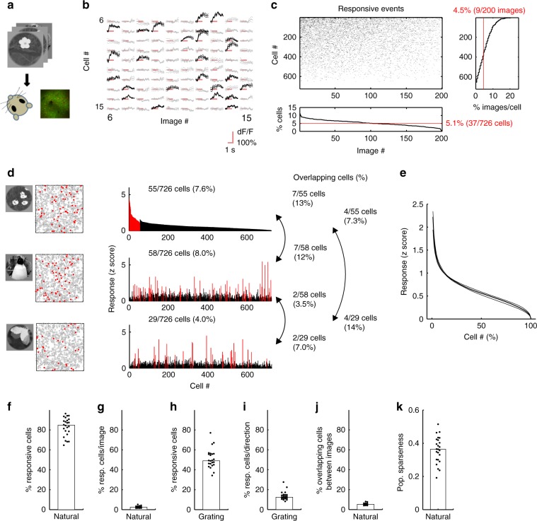
Natural scenes sparsely activate neurons in the primary visual cortex (V1). However, how sparsely active neurons reliably represent complex natural images and how the information is optimally decoded from these representations have not been revealed. Using two-photon calcium imaging, we recorded visual responses to natural images from several hundred V1 neurons and reconstructed the images from neural activity in anesthetized and awake mice. A single natural image is linearly decodable from a surprisingly small number of highly responsive neurons, and the remaining neurons even degrade the decoding. Furthermore, these neurons reliably represent the image across trials, regardless of trial-to-trial response variability. Based on our results, diverse, partially overlapping receptive fields ensure sparse and reliable representation. We suggest that information is reliably represented while the corresponding neuronal patterns change across trials and collecting only the activity of highly responsive neurons is an optimal decoding strategy for the downstream neurons.

Fig. 1. Sparse visual responses to natural images.

a Experimental schematic. Natural images are presented, and the activity of V1 neurons was recorded using two-photon Ca²⁺ imaging. b Examples of trial-averaged visual responses. The three lines for each response indicate the mean and the mean ± S.E.M. Black: significant responses, gray: non-significant responses, and red: stimulus periods. c Significant response events in an example plane (upper left). Bottom: the percentage of responsive cells for each image. Right: the percentage of images to which each cell responded. Red lines (bottom and right) indicate median values. d Examples of population response patterns to three images. Left: stimulus images and the spatial distributions of cells in an imaging area (side length: 507 microns). The red-filled and gray open circles indicate the responsive and remaining cells, respectively. Right: histograms of the visual responses to images presented in the left panels. Cells are divided into responsive (red) and the remaining groups (black), and are sorted in each group by the response amplitude to the image presented in the top row. The cell number order is fixed among the three histograms. e Distribution of the amplitude of responses to single images. The cell # is sorted by the amplitude of the response to each image and averaged across images in a plane. After normalizing the cell # (x-axis), data were collected across planes. The median (thick line) and 25–75th percentiles (thin lines) are shown. f Percentages of visually responsive cells. g Percentages of responsive cells per image. h Percentages of responsive cells for the moving grating. i Percentages of responsive cells for each direction of the moving grating. j Percentages of overlap of responsive cells between the natural images. k Population sparseness. f–k Each dot indicates data obtained from one plane, and the medians across planes are shown as bars. e–g, j, k N = 24 planes. h, i N = 23 planes (one plane data were discarded because of FOV drift during imaging). The stimulus images in a and d are adapted from the databases in refs. ^, with permission. Source data are provided as a Source Data file.

Fig. 2. Small overlap in visual features among neurons.

a Schematic of the transformation between a natural image and Gabor feature values. Each natural image was subjected to Gabor filters to obtain the feature values. Conversely, a set of feature values was transformed into an image. b Schematics of the Gabor filters. c Schematic of the encoding model. Ii, stimulus image in the ith trial. Gj: the jth Gabor filter. F_ji: the jth feature value obtained from Ii. W_j, the weight for the jth Gabor feature; R_i, the predicted visual response to Ii. d, e Response prediction in two neurons. Left: comparison between the observed and predicted responses. Right: weight parameters. The weights of one of ten models (each model corresponds to one of the ten-fold CVs) are shown. Insets: Forward filters (weighted sums of Gabor filters; red: positive values; blue: negative values). f The observed responses against the responses predicted by the linear step without nonlinear (NL) scaling in the neuron shown in (e). Red: NL scaling function curve. g NL scaling curves across planes. Gray: the averaged NL scaling curve across cells in each plane. Red: the averaged curve across planes (n = 24 planes). f, g The black line indicates y = x. h Upper left: Raster plot of the weights in the plane illustrated in Fig. 1c (red: positive weights, blue: negative weights). The median values for the models of the 10-fold CVs are shown. Right: the number of features used for each cell. Bottom: the percentage of cells for which each feature was used in the response prediction. Colored bar: the SF of the features. Red lines: median values. Half of the Gabor features are shown for visibility, but the remaining features were included in the data shown in the right panel. i Distribution of the number of features in each cell (n = 12,755 cells). j Distribution of the percentages of features that overlapped between cells (n = 3,993,653 cell pairs). d–f Each dot indicates a response to one image. The stimulus images in a and c are adapted from the database in ref. with permission. Source data are provided as a Source Data file.

Fig. 3. Image reconstruction from population activity.

a, b Schematic of the image reconstruction models. a In the all-cell model, each feature value was reconstructed by all cells. In the cell-selection model, the feature value was reconstructed by selected cells for each feature. The cell selection was based on the response prediction model for each cell; each cell participates in the reconstruction of features that the cell encodes in the response prediction model. b Details of the image reconstruction model. For each Gabor feature, j, feature values (F_ji, i: trial number across stimuli and trials, j: Gabor feature number) were independently regressed (weights: H_jk, k: cell number) by multiple cell responses (R_ki) to the image (Ii) in the ith trial. Then, a set of reconstructed features (F_1i, F_2i, …, F_1248i) was transformed into an image $\left({\widehat{\mathrm{I}}}_i\right)$. The flow of the reconstruction model is represented by black arrows from the bottom to the top. c Examples of reconstructed images from the main datasets (dataset 1; 200 images). Stimulus images presented during imaging (top), images that were reconstructed using the all-cell model (all cell, middle) and using the cell-selection model (cell selection, bottom) are shown. Each reconstructed image was averaged across trials. The reconstruction performances (R and CD) were computed for each trial, and trial-averaged performances are presented below each reconstructed image. d Examples of reconstructed images from other datasets (dataset 2; 1000–2000 images). e Distributions of R (top) and CD values (bottom) for the all-cell model (black lines) and the cell-selection model (red lines) in the example plane shown in Figs. 1 and 2 (n = 200 images reconstructed using 726 cells from a plane). Vertical lines indicate median values. f, g R f and CD g of dataset 1 (black lines and bars) and of dataset 2 (green lines) across planes. *p = 0.006 in f and p = 1.8 × 10⁻⁵ in g using the signed-rank test (n = 24 planes for dataset 1). Some of the stimulus images in b–d are adapted from the databases in refs. ^– with permission. Source data are provided as a Source Data file.

Fig. 4. Image reconstruction by a small number of responsive neurons.

a–c Top: examples of reconstructed images from a subset of responsive cells and from all cells. First panel: stimulus images. second–forth panels: reconstructed images from a subset of or all cells. Middle and bottom: reconstruction performances (middle, R; bottom, CD) plotted against the number of cells used for the reconstructions. The cells were first collected from the responsive cells (red dots) and then from the remaining cells (black dots). Horizontal lines: the performance from all cells. Vertical lines: the number of cells required for peak performance among all responsive cells. d, e Average performance curve (d R; e CD) plotted against the number of cells. Thick and thin lines indicate the means and the means ± S.E.M, respectively. f The contributions of the top 16 responsive cells to the image reconstruction shown in a. Top: reverse filters multiplied by the visual responses. Bottom: reconstructed images. g, h Left: median performances (g R; h CD) obtained from all cells (All), responsive cells (Resp.) and cells with peak performance (Max.). Right: the number of cells used for the reconstruction. (g left) p = 5.4 × 10⁻⁵ for Max. vs. Resp.; p = 1.2 × 10⁻⁴ for Resp. vs. All; p = 6.2 × 10⁻⁵ for Max. vs. All. (g right) p = 5.4 × 10⁻⁵. (h left) p = 5.4 × 10⁻⁵ for Max. vs. Resp.; p = 3.3 × 10⁻⁴ for Resp. vs. All; p = 1.3 × 10⁻⁴ for Max. vs. All. (h right) p = 1.7 × 10⁻⁵ using the signed-rank test. Each line indicates data for each plane, and bars indicate medians. Data for images that had at least ten responsive cells were used. i–k Weight overlap (i.e., features) between the cells that responded to the same image. i Schematic of the analysis. j Percentages of overlapping features for all-cell pairs responding to the same image. k The median percentages of overlapping features for all planes. Each dot indicates the median in each plane. d, e, g, h, k N = 24 planes. The stimulus images in a–c are adapted from the databases in ref. and with permission. Source data are provided as a Source Data file.

Fig. 5. Robustness of image representation against cell drop.

a Representative reconstructed images after dropping a single cell. Top panels: stimulus and reconstructed image obtained from all responsive neurons (55 cells). Middle panels: reconstructed images obtained after dropping a single cell. Bottom panels: representation patterns (reverse filters) of the dropped cells. The cell number (cell #) is the same as shown in Fig. 4f. b Reduction in reconstruction performance after removing a single cell. The cell #s on the x-axis are ordered from largest to smallest response amplitudes. The cell #s are in the same order as shown in Fig. 4d, e. Thick line: median. Thin lines: 25th and 75th percentiles; N = 24 planes. c Top panels: reverse filters of overlapping cells (nine example cells). The representation area of each neuron is contoured by the red line and overlaid on the right panel. Middle panel: reconstructed image obtained from the nine overlapping cells. Bottom panels: reconstructed images obtained from single cells (upper panels) and reconstructed images after dropping a single cell (lower panels). Dropping a single cell exerted only a small effect on the reconstructed images. d Representative reconstructed images obtained during the sequential dropping of the nine overlapping neurons. Cyan dotted lines indicate the overlapping area of the nine cells. The quality of the reconstructed image around the overlapping areas gradually degrades after each cell is dropped. e, f Plot of the R (or normalized R) for a local part of the reconstructed image (overlapping area) against the number (or percentage) of dropped cells for the representative case shown in c, e and for the summary of all data f. Data were collected and averaged across cells and across stimuli in each plane and then collected across planes. Thick lines: medians. Thin lines: 25th and 75th percentiles obtained across repetitions of random drops (n = 120 repetitions, e) or across planes (n = 24 planes, f). The stimulus images in a and d are adapted from the database in ref. with permission. Source data are provided as a Source Data file.

Fig. 6. Reliable image representation across trials.

a Examples of single-trial reconstructed images (top) and response patterns in a FOV (bottom). The first panel is a stimulus image, and the last panel is a trial-averaged image. FOV size: 507 micron each side. The color code for each dot indicates the response amplitude of each cell. b Single-trial evoked responses to the image in a. c Across-trial similarity of the reconstructed images (left) and the response patterns of responsive cells (right). The across-trial similarity was the Pearson’s correlation coefficient between a single-trial reconstructed image (or response pattern) and their trial average. d Across-trial variability of the reconstructed images (left) and the response patterns of responsive cells (right). The normalized squared error between a single-trial image (or response pattern) and their trial average was computed for the across-trial variability. e Reconstructed image from a set of overlapping cells (cell #1–9 in b). Upper left: stimulus image and trial-averaged reconstructed images from the nine overlapping cells. Cyan dotted line: the overlapping area. Upper right: representation (reverse filters) of the overlapping cells. Red line: the representation area. Cell #1 was the reference cell. Lower: single-trial representation patterns of three example cells (cell #1, 2, and 3) selected from the overlapping cells. Bottom: single-trial reconstructed images (upper) and single-trial response patterns in an FOV (lower) obtained from the nine overlapping cells. The brightness of each color dot in the lower panels indicates response amplitude of each cell. f Across-trial variability of a local part of reconstructed image (cyan dotted line in e) against the number of overlapping cells used for the reconstruction in the example case in e. Thick and thin lines are the median and 25th or 75th percentile, respectively (n = 200 random sequences of cell adding). g Across-trial variability against the percentage of overlapping cells used for the reconstruction. Black lines: raw data. Orange lines: trial-shuffled data. Thick and thin lines are median and 25th or 75th percentile, respectively. c, d, g N = 24 planes. The stimulus images in a and e are adapted from the database in ref. with permission. Source data are provided as a Source Data file.

Fig. 7. Representation of multiple images in a population.

a Schematic of the analysis. Responsive neurons (open and closed circles) were plotted for each image. Closed circles: responsive cells plotted for the first time for image N. Open circles: responsive cells that had already been plotted for image 1 – (N − 1). N, image number. b Raster plots of responsive cells for each image in the representative plane shown in a (n = 655/726 responsive cells). The image #s are sorted by the reconstruction performance (right panel). For each line, cells that did not respond to the previously plotted images are added to the right side. As the image # increases, the number of newly added cells decreases, and the cell # quickly reaches a plateau, indicating that many images are represented by a combination of cells that responded to other images. c, d The number of responsive cells (black line) and of newly added responsive cells (red line) are plotted against the image # for the case shown in b, c and averaged across planes d. The number of newly added cells quickly decreases as the image # increases. Three lines in each color indicate the mean and the mean ± S.E.M. e Schematic of the analysis. The feature set of each natural image was linearly regressed by the weights of the reconstruction model (the cell-selection model) from all the responsive cells in each plane. The weights of the reconstruction model were obtained based on a training dataset, and the target image was selected from a test dataset. The fitting error (%) was computed for each image. If the features encoded in all responsive cells were sufficient to represent natural images, the weights of the responsive cells should work as basis functions to represent the visual features of the natural images. f Distributions of the errors for all images in the example plane (shown in other figures). g The median error (%) across planes. Each dot indicates the median of each plane. d, g N = 24 planes. The stimulus image in e is adapted from the database in ref. with permission. Source data are provided as a Source Data file.

Fig. 8. Image representation in awake mice.

a, b Schematic of eye position analysis. a Image of a right eye. The white rectangle indicates the area recorded during imaging and analyzed offline (left). The recorded image (upper right panel) was binarized, and the pupil was fitted with an ellipse (red contour in lower right panel). The center of the ellipse was used to estimate the eye position (red dot). b Distribution map of eye position during imaging overlaid onto the image in a. The peak position of the distribution was detected, and the data were used for subsequent analyses only when the eye stayed around the peak position (white circle, <3.5 degrees or ~70 microns on the image). Scale bars: 1 mm. c Examples of eye position and locomotion state during imaging. Upper two panels: horizontal (X) and vertical (Y) eye positions. The red lines indicate time points at which the eye stayed around the peak position (inside the white circle in b). Lower two panels: position and velocity of a disc-type treadmill. The cyan lines indicate time points at which the mouse ran (velocity >2 cm/sec). d–h Image reconstruction by the cell-selection model in awake mice. d Examples of the reconstructed images. e, f Reconstruction performances (e pixel-to-pixel correlation, R. f coefficient of determination, CD); N = 7 planes. g, h R g and CD h versus the number of neurons. A single image was reconstructed by a small number of neurons. The thick black line and gray lines indicate the means and the means ± S.E.M, respectively (n = 6 planes). Only data for images that included at least five responsive cells were used. The stimulus images in d are adapted from the databases in refs. ^, with permission. Source data are provided as a Source Data file.

References

1. Rolls ET, Tovee MJ. Sparseness of the neuronal representation of stimuli in the primate temporal visual cortex. J. Neurophysiol. 1995;73:713–726. doi: 10.1152/jn.1995.73.2.713. - DOI - PubMed
1. Vinje WE, Gallant JL. Sparse coding and decorrelation in primary visual cortex during natural vision. Science. 2000;287:1273–1276. doi: 10.1126/science.287.5456.1273. - DOI - PubMed
1. Weliky M, Fiser J, Hunt RH, Wagner DN. Coding of natural scenes in primary visual cortex. Neuron. 2003;37:703–718. doi: 10.1016/S0896-6273(03)00022-9. - DOI - PubMed
1. Olshausen BA, Field DJ. Sparse coding of sensory inputs. Curr. Opin. Neurobiol. 2004;14:481–487. doi: 10.1016/j.conb.2004.07.007. - DOI - PubMed
1. Froudarakis E, et al. Population code in mouse V1 facilitates readout of natural scenes through increased sparseness. Nat. Neurosci. 2014;17:851–857. doi: 10.1038/nn.3707. - DOI - PMC - PubMed
Publication types
LinkOut - more resources