Topography in the Bursting Dynamics of Entorhinal Neurons

Abstract

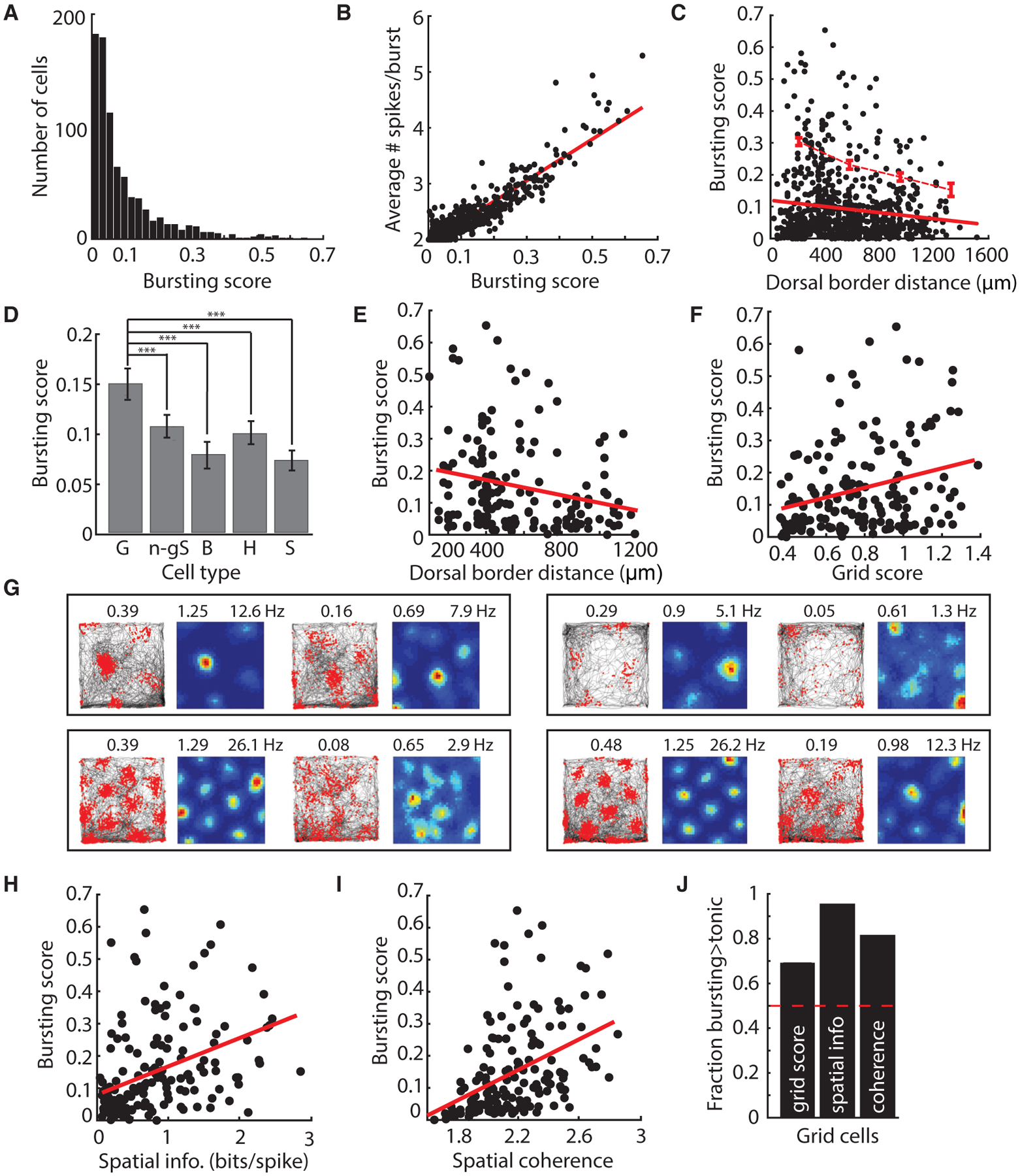
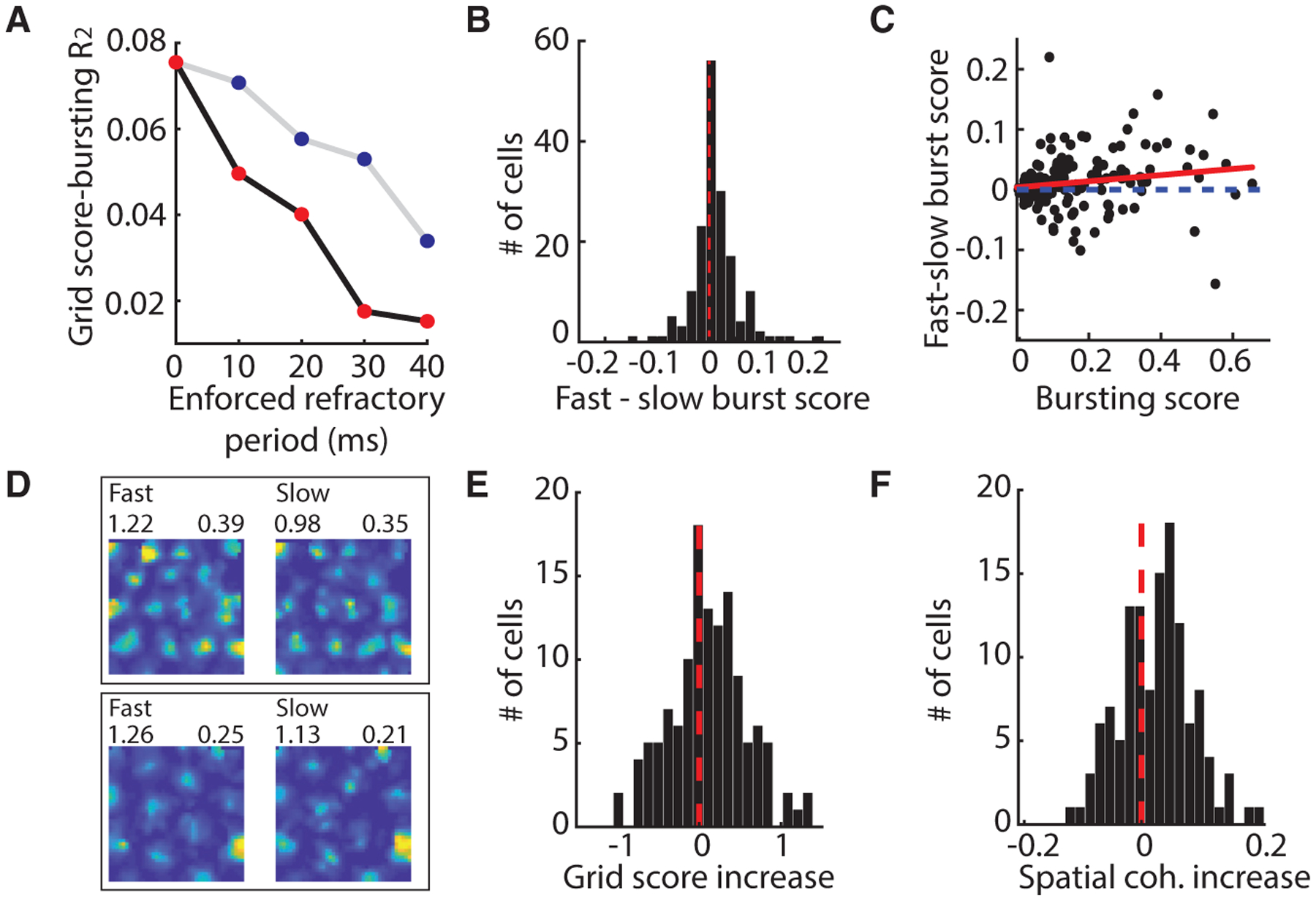
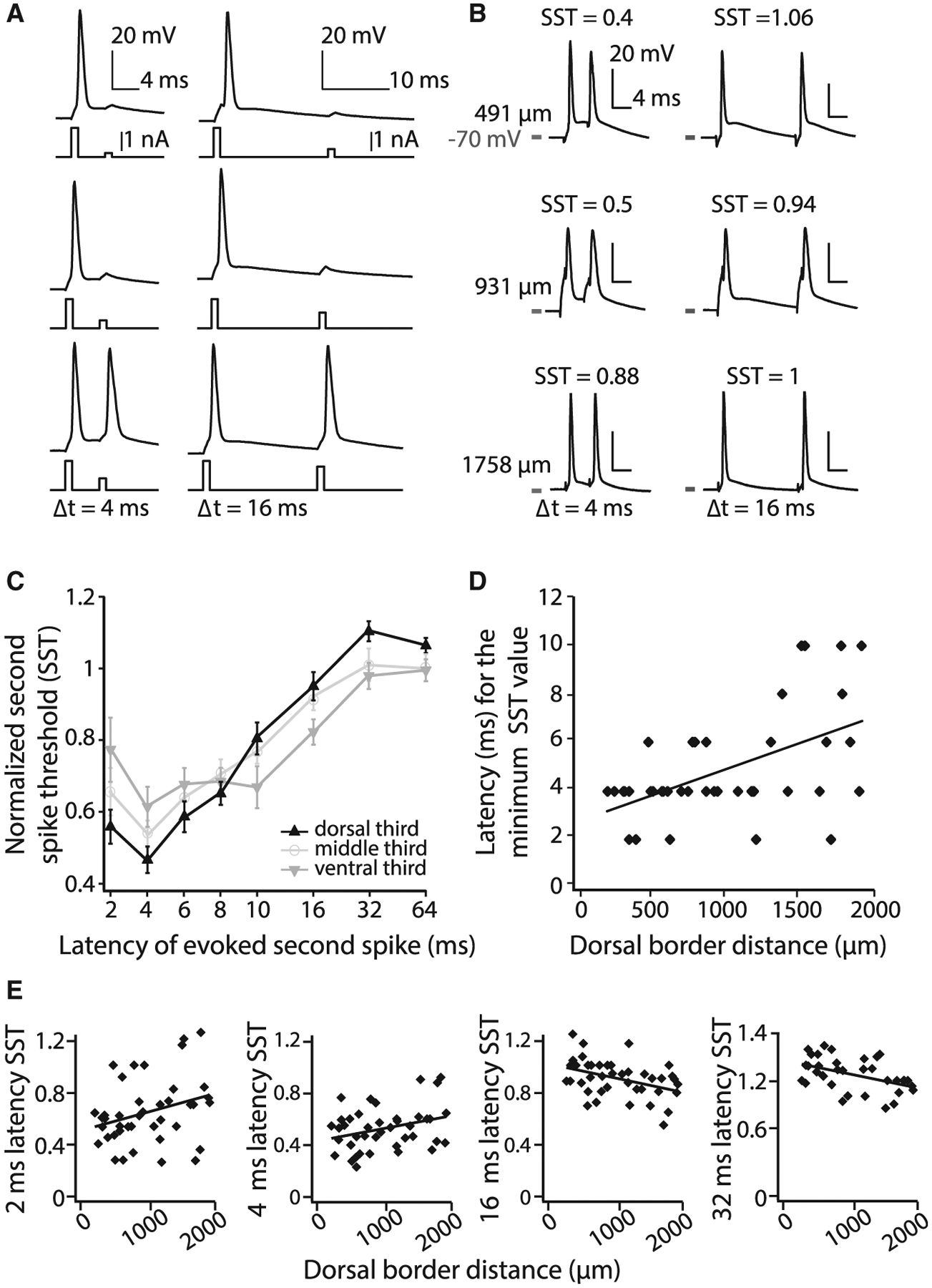
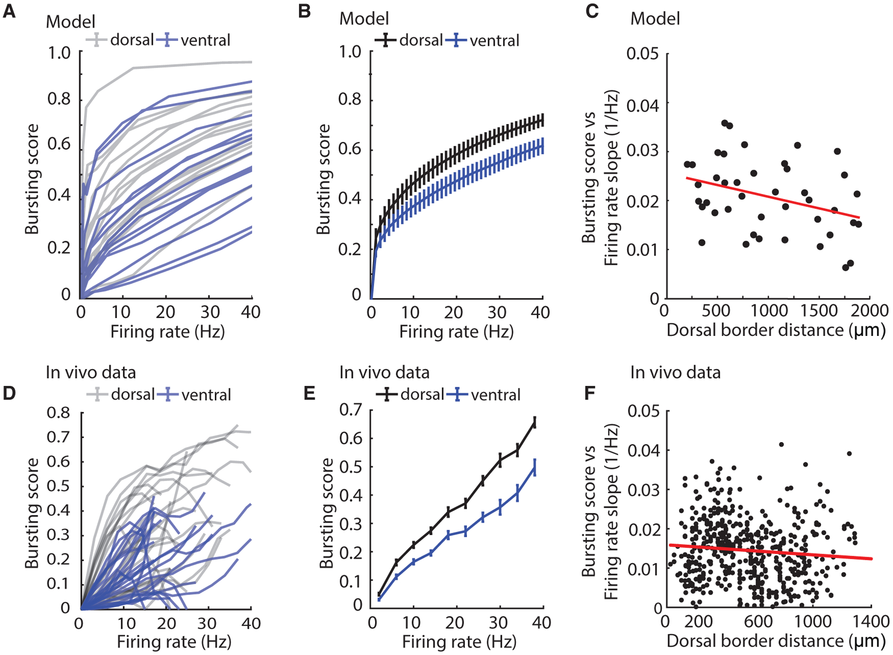
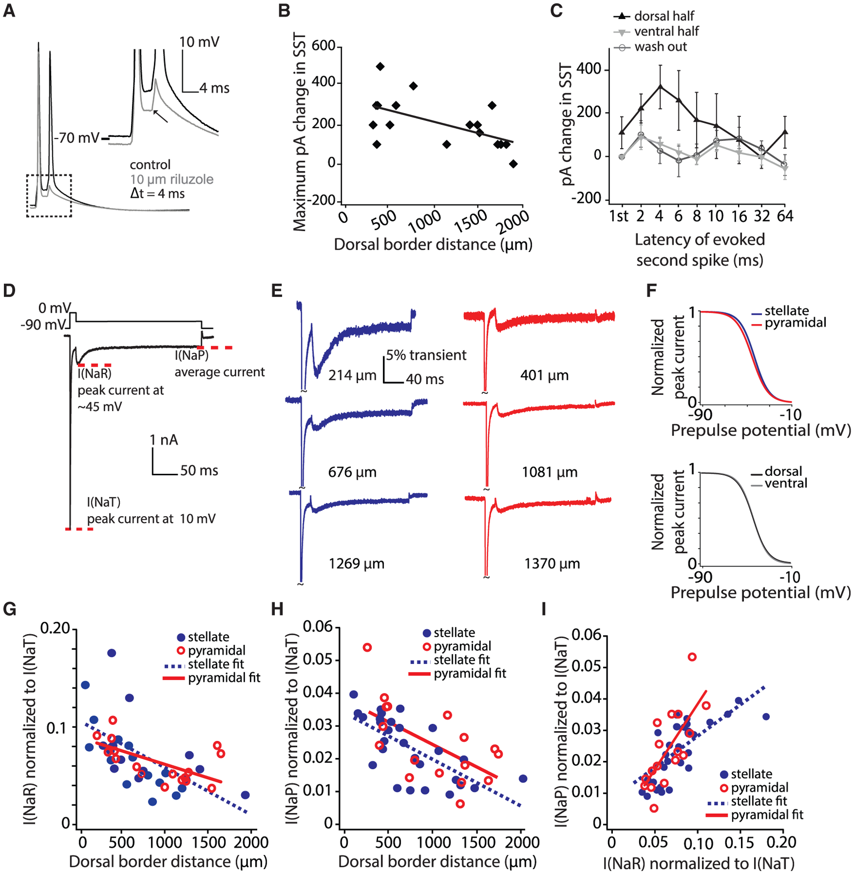
Medial entorhinal cortex contains neural substrates for representing space. These substrates include grid cells that fire in repeating locations and increase in scale progressively along the dorsal-to-ventral entorhinal axis, with the physical distance between grid firing nodes increasing from tens of centimeters to several meters in rodents. Whether the temporal scale of grid cell spiking dynamics shows a similar dorsal-to-ventral organization remains unknown. Here, we report the presence of a dorsal-to-ventral gradient in the temporal spiking dynamics of grid cells in behaving mice. This gradient in bursting supports the emergence of a dorsal grid cell population with a high signal-to-noise ratio. In vitro recordings combined with a computational model point to a role for gradients in non-inactivating sodium conductances in supporting the bursting gradient in vivo. Taken together, these results reveal a complementary organization in the temporal and intrinsic properties of entorhinal cells.

Figure 1.. In Vivo Bursting Dynamics Are Graded along the MEC DV Axis

(A) Histogram of BS for 821 MEC cells. (B) Average spikes per burst increased with BS. (C) BS decreases in a DV fashion among the top 25% of bursting scores (top dotted red line). Bottom red line indicates the linear fit for all cells. (D) Average BS ± SEM for grid (G), non-grid spatial (n-gS), border (B), head direction (H), and speed (S) cells. Grid cells showed higher BSs compared with other cell types (BS ± SEM: G = 0.15 ± 0.01, n-gS = 0.11 ± 0.01, B = 0.08 ± 0.01, H = 0.10 ± 0.01, S = 0.07 ± 0.01; one-way ANOVA: F[4, 856] = 10.9, p < 0.001; G versus n-gS, t[417] = 3.5, p < 0.001; B, t[251] = 4.3, p < 0.001; H, t[377] = 3.8, p < 0.001; S, t[309] = 5.7, p < 0.001). ***p < 0.001. (E and F) For grid cells, BS decreased with DV location (E) (BS × depth: R² = 0.056, p < 0.01), and grid score increased with BS (F) (BS × grid score: R² = 0.075, p < 0.01). Best-fit lines to data are in red. BS was significantly predicted by grid score even when depth and average firing rate were taken into account (significant coefficient in linear model predicting BS from grid score, depth, average FR: t[163] = 3.55, p < 0.001). BS was not significantly predicted by grid score in a model for which BS was predicted from grid score, spatial information, spatial coherence, depth, and average firing rate (“full model”: grid score, t[163] = 1.08, p = 0.28). However, grid score correlated strongly with spatial information (p < 0.001) and spatial coherence (p < 0.001), which were significant in this same model. (G) Each box shows trajectory (left) and rate maps (right) for two co-recorded grid cells. Cells on the left exhibited higher BSs than cells on the right. BSs denoted above plots showing the animal’s trajectory (black) overlaid with spikes (red dots). The grid score (left) and maximum firing rate (right) are denoted above the rate map, color-coded for minimum (blue) and maximum (red) values. (H and I) For grid cells, spatial information (H) and spatial coherence (I) increased with BS (BS × spatial information, R² = 0.15, p < 0.001; BS × spatial coherence, R² = 0.19, p < 0.001). Best-fit lines to data are in red. BS was significantly predicted by spatial information and spatial coherence, when depth and average firing rate were taken into account (spatial information, t[163] = 10.5, p < 0.001; spatial coherence, t[163] = 6.1, p < 0.001). BS was significantly predicted by spatial information, but not spatial coherence, in the full joint model (“full model”: spatial information, t[163] = 5.61, p < 0.001; spatial coherence, t[163] = −1.08, p = 0.28), although spatial information and spatial coherence were strongly correlated (p < 0.001). (J) Grid score, spatial information, and coherence computed from burst spikes are larger than those computed from the same number of tonic spikes. See also Figures S1–S4.

Figure 2.. Bursting In Vivo Likely Reflects Large or High-Frequency Inputs

(A) The correlation between grid score and BS decreases when bursts are replaced by single tonic spikes and continues to decrease as the minimum refractory period used to define a burst is increased (black line, red dots). Transparent dots correspond to values for which the correlation is not significant. Random rejection of spikes does not decrease the correlation (gray line, blue dots). (B) The BS increased during fast speeds. (C) The increase in BS during fast-compared with slow-speed epochs increases with the BS of a cell. Best-fit line to data is in red. (D) Firing rate maps of grid cell firing during fast (left) and slow (right) epochs color-coded for minimum (blue) and maximum (red) values. Grid score (top left) and BS (top right). (E and F) Grid score (E) and spatial coherence (F) increase during fast epochs. See also Figures S1–S4.

Figure 3.. In Vitro Bursting Dynamics Vary along the DV Axis of MEC

(A) Illustration of the current-clamp assay used to quantify the propensity to burst. The current required to evoke a spike is empirically determined and used as the first stimulus. The second 1 ms pulse (shown for two of eight latencies) is then increased in 100 pA increments until the cell reliably fires a second action potential. (B) Examples of the dual-pulse protocol at three latencies in three cells located along the DV axis (DV depth noted to the left and SST values at the top of each trace). (C) SST values for different latencies (log axis). Mean ± SEM plotted. The DV axis is binned into thirds (range 254–1,885 μm). Only cells in which all eight latencies were tested were included in this analysis. (D) For each cell, the latency at which the lowest SST value was measured is plotted relative to the cell’s position along the DV axis. Best-fit line to data is shown. (E) SST values for individual cells at different DV depths at four latencies. Best-fit lines to data are shown. See also Figure S5.

Figure 4.. Model Captures In Vivo Bursting Using Measured In Vitro Temporal Dynamics

(A) Bursting score versus firing for modeled cells on the basis of in vitro SST recordings and slow exponential decay times (simulations based on values from most dorsal third of axis in gray and most ventral third of axis in blue). (B) Summary data for dorsal and ventral thirds of modeled cells. (C) Slope of linear fit to all modeled single-cell curves in (A) as a function of dorsal border distance. (D) Bursting score versus firing rate for a random sample of in vivo cells (gray, most dorsal third; blue, most ventral third of axis). (E) Summary bursting score versus firing rate tuning curves for dorsal and ventral thirds of all in vivo cells (dorsal, n = 122; ventral, n = 90). Mean ± SEM plotted. (F) Slope of linear fit to all single-cell curves in (D) as a function of dorsal border distance. See also Figure S5.

Figure 5.. Na Current Components Are Graded along the MEC DV Axis

(A) A representative SST protocol recording in control (black) and riluzole (gray). Inset depicts the decrease in depolarization following a spike in the presence of riluzole. (B) Largest change (across all latencies) in the SST value in riluzole as a function of the cell’s position along the DV axis. Current plotted (pA) indicates the additional current required to rescue a second spike at a given latency. Best-fit line to data is shown. (C) Increase in picoamperes required to rescue control SST values at various latencies (log axis). Mean ± SEM plotted. The DV axis is binned into halves (dorsal, 315–1,139 μm; ventral, 1,140–1,885 μm). Only cells for which data on all eight latencies were obtained were included in this analysis. (D) Voltage-clamp protocol used to assay Na current components. The transient current is measured as the peak current elicited at 10 mV. I(NaR) is measured as the peak current elicited by any voltage repolarization. I(NaP) is measured as the average of the last 10 ms of the step. (E) Representative voltage-clamp recordings of stellate (blue) and pyramidal (red) neurons (DV location listed to the right of each trace). (F) Normalized Boltzman equation-derived steady-state inactivation curves plotted for average values from individual fits. Top shows stellate (blue) versus pyramidal (red) neurons and bottom shows dorsal (black) and ventral (gray) neurons. Four cells with insufficient traces were not included in this analysis. Na gradients did not show significant differences in inactivation parameters between stellate and pyramidal cells (mean ± SEM; V1/2, stellate = −42.7 ± 1.1 mV, pyramidal = −44.7 ± 1.2 mV, t[39] = 1.17, p = 0.25; slope factor (k), stellate = 6.41 ± 0.17 mV, pyramidal = 6.87 ± 0.15 mV, t[39] = −1.46, p = 0.15; Imax, stellate = −5.84 ± 0.33 nA, pyramidal = −4.67 ± 0.33 nA, t[39] = −0.99, p = 0.33). Inactivation parameters also did not differ between dorsal (0–1,000 μm) and ventral (>1,000 μm) cells (mean ± SEM; V1/2, dorsal = −43.4 ± 1.1 mV, ventral = −43.7 ± 1.2 mV, t[39] = 0.13, p = 0.90; slope factor (k), dorsal = 6.45 ± 0.16 mV, ventral = 6.80 ± 0.29 mV, t[39] = −1.14, p = 0.26; Imax, dorsal = −4.92 ± 0.40 nA, ventral = −5.30 ± 0.48 nA, t[39] = 0.61, p = 0.54). (G) Normalized I(NaP) density in stellate (blue) and pyramidal (red) neurons decreases along the DV axis. Best-fit lines to data are shown. (H) Same as (F) but for normalized I(NaP). The gradients of Na current component amplitudes did not differ between cell types (ANCOVA, comparison of slopes: I[NaP], F[1, 41] = 0.017, p = 0.90, η² = 0; I[NaR], F[1, 41] = 1.98, p = 0.17, η² = 0.05). (I) Correlation of I(NaR) and I(NaP) within individual neurons. Best-fit lines to data are shown. See also Figure S5.

References

1. Alonso A, and Klink R (1993). Differential electroresponsiveness of stellate and pyramidal-like cells of medial entorhinal cortex layer II. J. Neurophysiol 70, 128–143. - PubMed
1. Alonso A, and Llinás RR (1989). Subthreshold Na+-dependent theta-like rhythmicity in stellate cells of entorhinal cortex layer II. Nature 342, 175–177. - PubMed
1. Aman TK, Grieco-Calub TM, Chen C, Rusconi R, Slat EA, Isom LL, and Raman IM (2009). Regulation of persistent Na current by interactions between beta subunits of voltage-gated Na channels. J. Neurosci 29, 2027–2042. - PMC - PubMed
1. Azouz R, Jensen MS, and Yaari Y (1996). Ionic basis of spike after-depolarization and burst generation in adult rat hippocampal CA1 pyramidal cells. J. Physiol 492, 211–223. - PMC - PubMed
1. Bant JS, and Raman IM (2010). Control of transient, resurgent, and persistent current by open-channel block by Na channel beta4 in cultured cerebellar granule neurons. Proc. Natl. Acad. Sci. U S A 107, 12357–12362. - PMC - PubMed
Publication types
LinkOut - more resources