Hierarchical chromatin organization detected by TADpole

Abstract

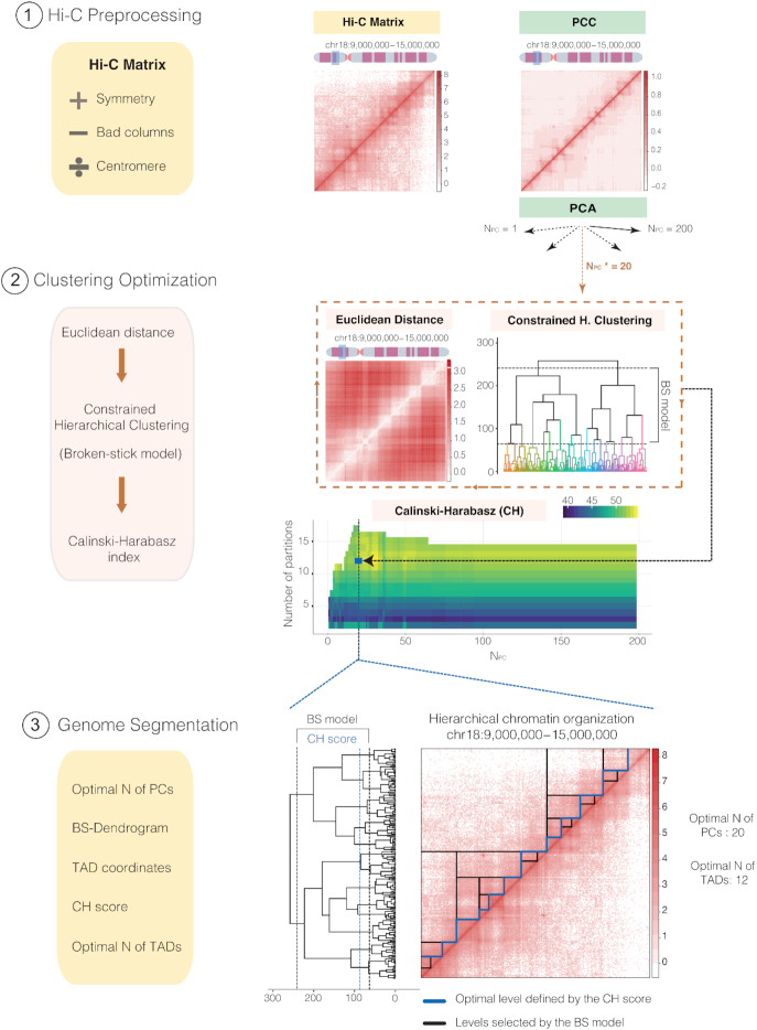
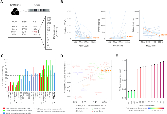
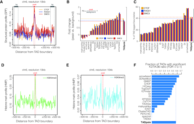
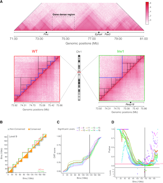
The rapid development of Chromosome Conformation Capture (3C-based techniques), as well as imaging together with bioinformatics analyses, has been fundamental for unveiling that chromosomes are organized into the so-called topologically associating domains or TADs. While TADs appear as nested patterns in the 3C-based interaction matrices, the vast majority of available TAD callers are based on the hypothesis that TADs are individual and unrelated chromatin structures. Here we introduce TADpole, a computational tool designed to identify and analyze the entire hierarchy of TADs in intra-chromosomal interaction matrices. TADpole combines principal component analysis and constrained hierarchical clustering to provide a set of significant hierarchical chromatin levels in a genomic region of interest. TADpole is robust to data resolution, normalization strategy and sequencing depth. Domain borders defined by TADpole are enriched in main architectural proteins (CTCF and cohesin complex subunits) and in the histone mark H3K4me3, while their domain bodies, depending on their activation-state, are enriched in either H3K36me3 or H3K27me3, highlighting that TADpole is able to distinguish functional TAD units. Additionally, we demonstrate that TADpole's hierarchical annotation, together with the new DiffT score, allows for detecting significant topological differences on Capture Hi-C maps between wild-type and genetically engineered mouse.

Figure 1.

General overview of TADpole tool. Schematic overview of the TADpole algorithm. (1) TADpole input is an all-versus-all tab-limited Hi-C matrix. The matrix is checked for symmetry and low-quality columns (called as bad columns—BC) are removed. Large matrices of entire chromosomes are optionally split at the centromere to create two smaller sub-matrices corresponding to the chromosomal arms. Next, matrix denoising and dimensionality reduction take place by computing the corresponding PCC matrix, and by performing a PCA on it. (2) Per each number of first PCs retained (from 1 to 200), the corresponding PC matrix is transformed into its Euclidean distance matrix (EDM). The EDM serves as the input to perform the constrained hierarchical clustering (CH-clust). The range of significant hierarchical levels is fixed from level 1 (corresponding to partitioning the region into 2 TADs) up to an upper bound given by the broken-stick model (BS), then the Calinski-Harabasz (CH) index is used to select the optimal level. (3) As output, TADpole returns the optimal number of first PCs (N_pc*) retained to obtain the optimal set of TADs, the dendrogram with the significant hierarchical levels, the coordinates of the chromatin domains for each level with its associated CH index, and the optimal number of TADs. A real example of TADpole tool applied to a 6Mb-region (chr18:9,000,000–15,000,000) of a human Hi-C dataset (HIC003; SRR1658572) at 30 kb resolution obtained from Rao et al. (15). Two bad columns were detected and removed from the input data and then, the PCC and the PCA were computed (using the first 200 PCs). Using the first 20 PCs, the EDM is computed and is used as the input for the CH-clust. A total of 16 hierarchical levels are retrieved according to the BS model and, for each one, the CH index is computed (this process is repeated iteratively for each set of PCs analyzed). This step produces a matrix of CH indexes (with the result of the 200 computed dendrograms) from which the highest average score is selected (highlighted with the blue square), in this case corresponding to 12 TADs and the first 20 PCs (N_pc*). Taking these values, a complete dendrogram of the Hi-C matrix is retrieved, cut using the broken-stick model to select significant levels (containing from 2 to 17 TADs, shown between black lines) and, from them, the highest-scoring level according to the CH index is selected (blue line). On the right, the Hi-C contact map is presented showing the complete hierarchy of the significant levels selected by the BS model (black lines) along with the optimal one in 12 specific TADs, as identified by the highest CH index (blue line).

Figure 2.

Technical benchmarking of TADpole. (A) General overview of the dataset used for the technical benchmarking analysis from Zufferey et al. (29). The dataset includes the Hi-C interaction matrix of chromosome 6 in GM12878 cells in 24 different forms (‘Materials and Methods’ section). (B–E) Results of the technical benchmarking of TADpole considering the optimal level with its corresponding TADs in each case and comparing with the other 22 TAD callers considered in Zufferey et al. (29). (B) The number, and the size of TADs in kilobases (kb) and number of bins. Each gray line represents each one of the other 22 TAD callers. (C) Percentage of conserved TADs boundaries over different resolutions across the 22 TAD callers. (D) The average MoC values across normalization strategies against the average MoC values across resolutions. Colors group the different TAD callers according to their specific mathematical approach. (E) MoC values for different down-sampling matrices from the ICE-normalized interaction matrix at 50kb of resolution. Panels B–D have been adapted from Figures 2C, 1D-E and Supplementary S2B of Zufferey et al. (29) to include TADpole in the comparison of TAD callers.

Figure 3.

Biological benchmarking of TADpole. TAD boundaries used in these analyzes are the result of the optimal TAD partition defined by TADpole of the Hi-C matrix at 10 kb of resolution. (A) SPP around the TAD boundaries (peak region in red, background region in gray) are shown for the consensus profile of CTCF, RAD21 and SMC3. (B) Fold-change of the SPP of CTCF, RAD21 and SMC3 at TAD boundaries for all the 22 TAD callers. (C) Percentage of TAD boundaries hosting CTCF, RAD21 and SMC3 for all the TAD callers. (D andE) HMP computed around TAD boundaries for active promoter mark (H3K4me3) and repressive histone mark (H3K9me3). (F) The fraction of TADs with significant log10 ratio between H3K27me3 and H3K36me3 obtained for TADpole and for other 22 TAD callers. Panels B, C and F have been adapted from Figure 5D, E, I from Zufferey et al. (29).

Figure 4.

Characterization of topological difference in capture Hi-C datasets. (A) Top: Overview of the entire WT captured region (chr1:71.00–81.00Mb) in Kraft et al. (42). The gene-dense region harbors the breakpoint of the inversion (Inv1). Bottom: Capture Hi-C maps of the gene-dense region (chr1:73 920 000–75 860 000) in WT and inversion 1 (Inv1) strains. In both matrices, the significant hierarchical levels are shown as black lines and the optimal one as a blue line. (B) Example of DiffT score for the ninth hierarchical level (corresponding to 10 TADs) of the dendrogram. The upper triangle of the matrix shows the TADs identified by TADpole in WT and Inv1 matrices as red and green continuous lines, respectively. The lower triangle of the matrix shows the conserved (in orange) and non-conserved (in gray) areas of the TADs. In the panels C and D, the Inv1 breakpoint is highlighted with a solid black line, and only the levels that contain at least one bin with a DiffT-score associated P-value < 0.05, are shown. (C) DiffT score profiles as a function of the matrix bins. The calculation of the DiffT score is used to obtain a curve in panel C from the TAD partition in panel B is illustrated in Supplementary Video S1. (D) P-value profiles per bin for automated detection of significant differences. In the lower panel, the bins associated with minimum P-values per level are marked with empty dots.

References

1. Sexton T., Cavalli G.. The role of chromosome domains in shaping the functional genome. Cell. 2015; 160:1049–1059. - PubMed
1. Dekker J., Mirny L.. The 3D genome as moderator of chromosomal communication. Cell. 2016; 164:1110–1121. - PMC - PubMed
1. Stadhouders R., Vidal E., Serra F., Di Stefano B., Le Dily F., Quilez J., Gomez A., Collombet S., Berenguer C., Cuartero Y. et al. .. Transcription factors orchestrate dynamic interplay between genome topology and gene regulation during cell reprogramming. Nat. Genet. 2018; 50:238–249. - PMC - PubMed
1. Paulsen J., Liyakat Ali T.M., Nekrasov M., Delbarre E., Baudement M.O., Kurscheid S., Tremethick D., Collas P.. Long-range interactions between topologically associating domains shape the four-dimensional genome during differentiation. Nat. Genet. 2019; 51:835–843. - PubMed
1. Bonev B., Mendelson Cohen N., Szabo Q., Fritsch L., Papadopoulos G.L., Lubling Y., Xu X., Lv X., Hugnot J.P., Tanay A. et al. .. Multiscale 3D genome rewiring during mouse neural development. Cell. 2017; 171:557–572. - PMC - PubMed
Publication types