High-Accuracy Detection of Neuronal Ensemble Activity in Two-Photon Functional Microscopy Using Smart Line Scanning

Abstract

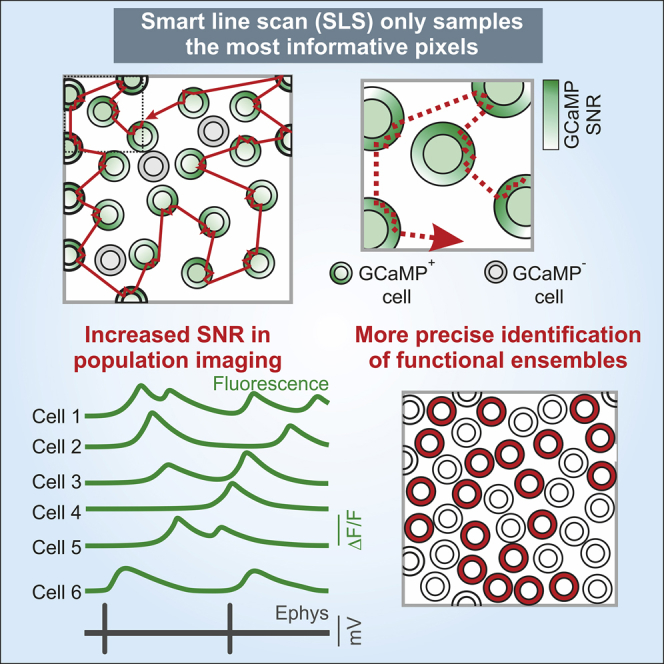
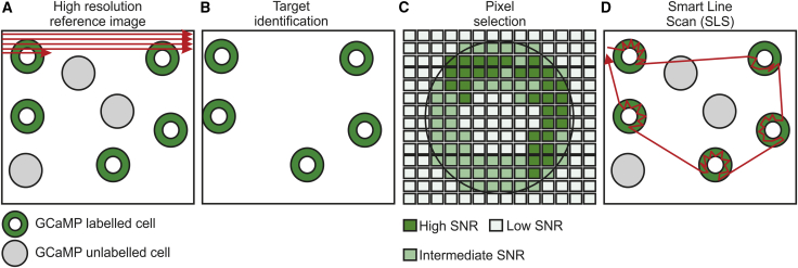
Two-photon functional imaging using genetically encoded calcium indicators (GECIs) is one prominent tool to map neural activity. Under optimized experimental conditions, GECIs detect single action potentials in individual cells with high accuracy. However, using current approaches, these optimized conditions are never met when imaging large ensembles of neurons. Here, we developed a method that substantially increases the signal-to-noise ratio (SNR) of population imaging of GECIs by using galvanometric mirrors and fast smart line scan (SLS) trajectories. We validated our approach in anesthetized and awake mice on deep and dense GCaMP6 staining in the mouse barrel cortex during spontaneous and sensory-evoked activity. Compared to raster population imaging, SLS led to increased SNR, higher probability of detecting calcium events, and more precise identification of functional neuronal ensembles. SLS provides a cheap and easily implementable tool for high-accuracy population imaging of neural GCaMP6 signals by using galvanometric-based two-photon microscopes.

Keywords: GCaMP6; barrel cortex; neuronal ensembles; spatiotemporal neural responses; two-photon imaging.

Graphical abstract

Figure 1

Schematic Representation of SLS (A) In raster scanning, images are generated scanning the excitation spot (red arrow) over all pixels in the FOV in a sequential raster trajectory. Fluorescence from GcaMP-labeled neurons (green), background structures (white), and GcaMP-unlabeled cells (gray) is sampled. (B) In SLS, scanned regions corresponding to labeled cells (green donuts) are identified based on the reference raster scan t-series. (C) Pixels belonging to one cell are sorted according to their SNR (green shades), and the subset of pixels maximizing the SNR is selected (ROIs). (D) SLS trajectories (red) intersect only selected pixels.

Figure 2

Pixel-Wise Statistics Identify the Subset of Most Informative Pixels to Scan Inside Each Cell (A) Two-photon raster scanning image showing layer IV neurons of the barrel cortex expressing GCaMP6s in an anesthetized mouse. Intensity projection of GCaMP6s fluorescence signal (gray scale) and SNR (pseudocolor scale) are shown. (B) Six cells in (A) are displayed at an enlarged scale. Color code as in (A). (C) Distribution of the SNR of cytoplasmic pixels (n = 164 cells from N = 8 mice). (D) Intensity projection of GCaMP6s signal (gray) of a t-series recorded in layer IV. The red cross indicates the center of the identified cell and the red box the boundaries of the region in which pixel-wise statistics are computed to identify ROIs. (E) Average SNR value as a function of the number of selected pixels for the cell showed in (D). Inset: four images of the cell highlighted in (D) are shown. Each image shows a different number of selected pixels (9, 46, 107, and 153, respectively). (F) Same FOV as in (D) after pixels selection. A total of 83 ROIs (red pixels) were identified.

Figure 3

Motion Artifacts in SLS (A) X and Y displacement during raster scanning in anesthetized animals (n = 3 mice, gray), quiet wakefulness (n = 3 mice, orange), and active wakefulness (n = 3 mice, magenta). (B) Top: representative SLS acquisition during active wakefulness. Pseudocolor scale indicates fluorescence amplitude. Middle: autoregressive second order fit (AR(2), red) of SLS PC1 (black). Bottom: cross correlation (green) between AR(2) and the PC1. The gray arrowhead indicates a movement artifact detected when the 0.3 threshold is crossed. (C) Representative SLS acquisition with no detected large motion artifacts during quite wakefulness. (D) Fluorescence over time without (no reassignment, gray) or with (reassigned, red) the reassignment of 11 pixels. (E) SNR as a function of the number of reassigned pixels for one representative ROI. The gray and the red asterisks indicate the conditions displayed in (D). (F) Correlation between the motion displacement calculated using NoRMCorre on the reference patch and the motion displacement computed from the pixels reassignment approach (black dots). Empty circles: individual experiments; filled circles: average ± SD. Data from the reference patch were downsampled in time before applying NoRMCorre. Motion displacement values were separately calculated for the X (left) and the Y (right) direction in the reference patch and in the ROIs. The correlation between the motion displacement calculated using NoRMCorre and a random pixels reassignment are shown in gray. Left: downsampling 0.5 Hz, p = 0.08; downsampling 1 Hz, p = 0.18; downsampling 2 Hz, p = 0.06; downsampling 5 Hz, p = 0.32; paired t test, n = 13 SLS acquisitions. Right: downsampling 0.5, p = 2E-6; downsampling 1 Hz, p = 2E-4; downsampling 2 Hz, p = 2E-5; downsampling 5 Hz, p = 8E-9; paired t test n = 13 SLS acquisitions. In this as well in other figures: *, p < 0.05; **, p < 0.01; ***, p < 0.001; n.s., non significant. Error bars represent ± SD.

Figure 4

Neuropil Decontamination in SLS (A) Left: a GCaMP6s-expressing layer IV cell. Right: the pixels belonging to the ROI (red), the local neuropil (green, local np), and the global neuropil (blue, global np) are shown. SLS trajectory is shown in yellow and pixels at the border between the ROI and the local np were not considered (white, skipped). (B) Black traces on the left: raw fluorescence signal over time from SLS on one representative cell (ROI), its corresponding local np, and the global np. Grey traces on the right: PC1 computed from the combined pixels of all the ROIs (upper trace), PC1 of all local np regions (middle trace), and PC1 of the whole global np (bottom trace). (C) Pearson’s correlation between the PC1 of the signal from local np regions and the PC1 of the global np regions as a function surround region dimension (from 0 to 3 pixels). n = 172 ROIs from 11 SLS for each surround region value; paired t test, p = 1E-11 for surround 1 pixel versus surround 2 pixel; p = 0.04 for surround 2 pixel versus surround 3 pixels; p = 2E-9 for surround 3 versus surround 4 pixels. (D) Pearson’s correlation between the PC1 of the ROI signal and the global np as a function of the surround region dimension (from 0 to 3 pixels). n = 90 ROIs from 5 SLS for each surround region value; paired t test, p = 0.1 for surrond 0 pixel versus surround 1 pixel; p = 0.1 for surround 1 pixel versus surround 2 pixels; p = 0.96 for surround 2 versus surround 3 pixels. (E) Left: raw fluorescence over time for four ROIs (black traces) acquired in SLS. Right: corrected fluorescence signals for the same four ROIs shown on the left after neuropil decontamination (gray traces). Neuropil correction is obtained subtracting from the raw fluorescence traces the weighted PC1 of the global np signal. (F) Pearson’s correlation across ROIs before (raw) and after neuropil decontamination using different strategies (global np subtraction, local np subtraction, and subtraction of the weighted PC1 of the global np). n = 3,656 ROI pairs from 11 SLS; Wilcoxon rank-sum test, p = 0.02 for raw versus global np subtraction; p = 2E-4 for raw versus local np subtraction; p = 0.02 for raw versus PC1 of the global np; p = 0.08 for global versus local np subtraction; p = 0.07 for global np versus PC1 of the global np subtraction; p = 0.01 for local np versus PC1 of the global np subtraction.

Figure 5

SLS Allows Single AP Resolution during Population Imaging (A) GCaMP6s-expressing layer IV principal neurons. Yellow circles identify 155 neurons. (A₁) SLS trajectory (yellow line) crossing all the identified cells. (B and B₁) Fluorescence over time from the two cells indicated in red in (A) in conventional raster scanning acquisitions (B) and SLS (B₁). Blue ticks above traces indicate whisker stimuli (duration: 200 ms). (C and C₁) Fluorescence over time of all cells shown in (A) (gray traces) during consecutive whisker stimulations and the average across cells (black trace) in raster scanning (C) and SLS (C₁). (D) SNR of events in all raster scan series and all SLS acquisitions. n = 360 cells from 4 animals; paired t test, p = 5E-4. (E) Fraction of cells responding to the whisker stimulation in raster scanning and SLS. n = 360 cells from 4 animals; paired t test, p = 4E-12. (F–F₃) Simultaneous juxtasomal recording and raster scan experiment from a GCaMP6s-expressing neuron at 10 Hz (F) and 30 Hz (F₁). The white line indicates the recording pipette. The same cell in (F) is recorded using juxtasomal recording and SLS imaging in a much larger FOV at 30 Hz (F₂) and 62.5 Hz (F₃). The yellow line in (F₂) and (F₃) represents the SLS trajectory across the different cells (white number). The same cells were differently numbered in SLS at 30 Hz and 62.5 Hz because the SLS trajectory changed when the surround region was modified to change the scanning rate. (G) Left: fluorescence over time acquired in raster scanning at 10 Hz (top) and electrophysiology recording (bottom). Right: fluorescence over time acquired in raster scanning at 30 Hz (top) and electrophysiology recording (bottom). (G₁) The same as in (G) for SLS at 30 Hz (left) and at 62.5 Hz (right). (H) SNR of fluorescence events associated to isolated APs (see STAR Methods) under the different conditions. n = 16 acquisitions from 8 FOVs in 4 animals; Wilcoxon rank-sum test; p = 5E-4 for raster scan at 10 Hz versus raster scan at 30 Hz; p = 0.12 for raster scan at 30 Hz versus SLS at 30 Hz; p = 7E-3 for SLS at 30 Hz versus SLS at 62.5 Hz. (I) Accuracy of single AP detection under the different conditions. n = 16 acquisitions from 8 FOVs in 4 animals; Wilcoxon rank-sum test; p = 2E-3 for raster scan at 10 Hz versus raster scanning at 30 Hz; p = 0.01 for raster scan at 30 Hz versus SLS at 30 Hz; p = 2E-3 for SLS at 30 Hz versus SLS at 62.5 Hz.

Figure 6

Increased Rate of Detected Neural Ensembles in SLS (A) Top: functional ensembles (red dots) detected in an awake animal using raster scan imaging (frame rate: 0.8 Hz). Bottom: functional ensembles (red dots) detected in the experiment shown in the top panel using SLS (frame rate: 48 Hz). The gray vertical shades indicate whisker stimuli. Blue dots indicate active neurons not belonging to any ensemble. (B and C) Rate of detected ensembles in anesthetized (B) and awake (C) animals under the different conditions. Data are classified according to modality (raster or SLS at different acquisition rates) and to the type of activity (spontaneous or air puff stimulation). Spontaneous activity in (B): n = 6 for raster, n = 6 for SLS at 0–20 Hz, n = 6 for SLS at 20–40 Hz, n = 3 for SLS at >40 Hz from 6 anesthetized mice. Paired t test, p = 0.01 for raster versus SLS 0–20 Hz, p = 3E-7 for raster versus SLS 20–40 Hz; unpaired t test, p = 6E-8 for raster versus SLS >40 Hz. Air puff stimulation in (B): n = 20 for raster, n = 15 for SLS at 0–20 Hz, n = 13 for SLS at 20–40 Hz, n = 7 for SLS at >40 Hz from 6 anesthetized mice. Unpaired t test, p = 1E-7 for raster versus SLS 0–20 Hz, p = 6E-8 for raster versus SLS 20–40 Hz, p = 6E-7 for raster versus SLS >40 Hz. Spontaneous activity in (C): n = 5 for raster and n = 4 for SLS at 0–20 Hz from 2 awake mice; unpaired t test, p = 4E-9. Air puff stimulation in (C): n = 7 for raster and n = 8 for SLS at 0–20 Hz from 2 awake mice; unpaired t test, p = 4E-9. (D and E) Same as in (B) and (C) but for SLS downsampled to match the acquisition frequency of raster scanning (Acq. freq. match). Spontaneous activity in (D): paired t test, p = 0.01 for raster versus SLS 0–20 Hz, p = 1E-4 for raster versus SLS 20–40 Hz; unpaired t test, p = 5E-5, for raster versus SLS >40 Hz. Air puff in (D): unpaired t test, p = 2E-6 for raster versus SLS 0–20 Hz, p = 7E-7 for raster versus SLS 20–40 Hz, p = 3E-5 for raster versus SLS >40 Hz. Spontaneous activity in (E): unpaired t test, p = 2E-7. Air puff stimulation in (E): t test, p = 3E-7. Unpaired t test, p = 0.01, for raster in spontaneous versus raster in air puff stimulation.

Figure 7

Increased Rate of Detected Calcium Events in SLS (A) Left: rate of detected calcium events in anesthetized animals under the different conditions. Right: rate of detected events with downsampling of SLS to match the acquisition rate of raster scanning. Spontaneous activity: n = 6 for raster, n = 6 for SLS at 0–20 Hz, n = 6 for SLS at 20–40 Hz, n = 3 for SLS at >40 Hz from 6 anesthetized mice. Left: paired t test, p = 0.32 for raster versus SLS 0–20 Hz, p = 4E-3 for raster versus SLS 20-40 Hz; unpaired t test, p = 1E-4 for raster versus SLS >40 Hz. Right: paired t test, p = 0.02 for raster versus SLS 0–20 Hz, p = 1E-4 for raster versus SLS 20–40 Hz; unpaired t test p = 1E-4 for raster versus SLS >40 Hz. Air puff stimulation: n = 20 for raster, n = 15 for SLS at 0–20 Hz, n = 13 for SLS at 20–40 Hz, n = 7 for SLS at >40 Hz from 6 anesthetized mice. Left: unpaired t test, p = 0.01 for raster versus SLS 0–20 Hz, p = 1E-4 for raster versus SLS 20–40 Hz, p = 1E-4 for raster versus SLS >40 Hz. Right: unpaired t test, p = 1E-4 for raster versus SLS 0–20 Hz, p = 3E-6 for raster versus SLS 20–40 Hz, p = 6E-8 for raster versus SLS >40 Hz. (B) Same as in (A) for awake mice. Spontaneous activity: n = 5 for raster and n = 4 for SLS at 0–20 Hz from 2 awake mice. Unpaired t test, p = 4E-6 and p = 9E-6 for left and right panels. Air puff stimulation: n = 7 for raster and n = 8 for SLS at 0–20 Hz from 2 awake mice. Unpaired t test, p = 2E-8 and p = 6E-8 for left and right panels. (C) Normalized amplitude of events under the different conditions in anesthetized mice. Same dataset as in (A). Spontaneous activity: paired t test, p = 6E-8 for raster versus SLS 0–20 Hz, p = 6E-8 for raster versus SLS 20–40 Hz; unpaired t test, p = 6E-8 for raster versus SLS >40 Hz. Air puff stimulation: unpaired t test, p = 6E-8 for raster versus SLS 0–20 Hz, p = 6E-8 for raster versus SLS 20–40 Hz, p = 6E-8 for raster versus SLS >40 Hz. (D) Same as in (C) for awake mice. Number of acquisitions for each condition as in (B). Spontaneous activity: unpaired t test, p = 2E-6. Air puff stimulation: unpaired t test, p = 1E-7.

References

1. Akemann W., Léger J.F., Ventalon C., Mathieu B., Dieudonné S., Bourdieu L. Fast spatial beam shaping by acousto-optic diffraction for 3D non-linear microscopy. Opt. Express. 2015;23:28191–28205. - PubMed
1. Bindocci E., Savtchouk I., Liaudet N., Becker D., Carriero G., Volterra A. Three-dimensional Ca2+ imaging advances understanding of astrocyte biology. Science. 2017;356:eaai8185. - PubMed
1. Bovetti S., Fellin T. Optical dissection of brain circuits with patterned illumination through the phase modulation of light. J. Neurosci. Methods. 2015;241:66–77. - PubMed
1. Bovetti S., Moretti C., Zucca S., Dal Maschio M., Bonifazi P., Fellin T. Simultaneous high-speed imaging and optogenetic inhibition in the intact mouse brain. Sci. Rep. 2017;7:40041. - PMC - PubMed
1. Bzdok D., Krzywinski M., Altman N. Machine learning: supervised methods. Nat. Methods. 2018;15:5–6. - PMC - PubMed
Publication types
LinkOut - more resources