. 2020 Jun 1;37(6):1819-1831.
doi: 10.1093/molbev/msaa049.

Relative Efficiencies of Simple and Complex Substitution Models in Estimating Divergence Times in Phylogenomics

Affiliations

Relative Efficiencies of Simple and Complex Substitution Models in Estimating Divergence Times in Phylogenomics

Qiqing Tao et al. Mol Biol Evol. .

Abstract

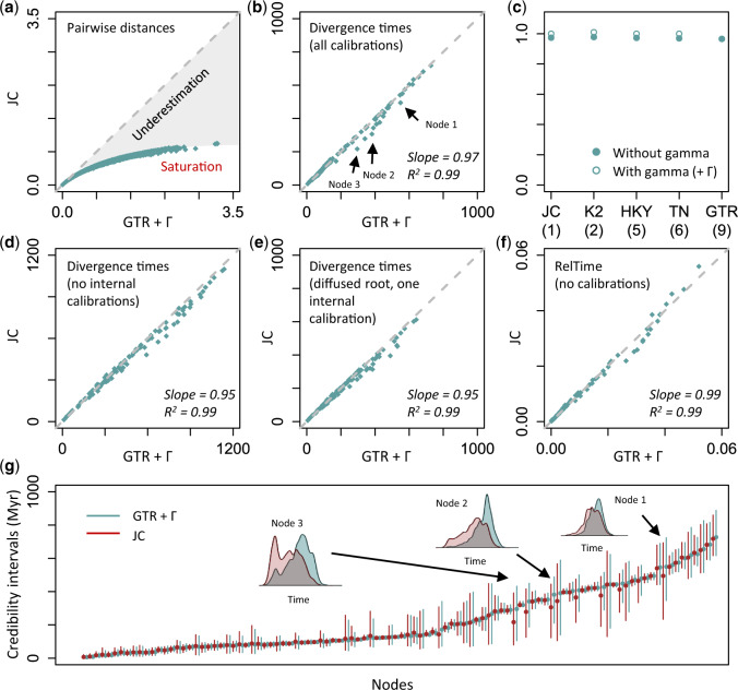
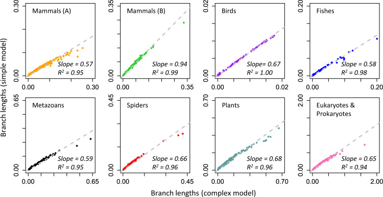
The conventional wisdom in molecular evolution is to apply parameter-rich models of nucleotide and amino acid substitutions for estimating divergence times. However, the actual extent of the difference between time estimates produced by highly complex models compared with those from simple models is yet to be quantified for contemporary data sets that frequently contain sequences from many species and genes. In a reanalysis of many large multispecies alignments from diverse groups of taxa, we found that the use of the simplest models can produce divergence time estimates and credibility intervals similar to those obtained from the complex models applied in the original studies. This result is surprising because the use of simple models underestimates sequence divergence for all the data sets analyzed. We found three fundamental reasons for the observed robustness of time estimates to model complexity in many practical data sets. First, the estimates of branch lengths and node-to-tip distances under the simplest model show an approximately linear relationship with those produced by using the most complex models applied on data sets with many sequences. Second, relaxed clock methods automatically adjust rates on branches that experience considerable underestimation of sequence divergences, resulting in time estimates that are similar to those from complex models. And, third, the inclusion of even a few good calibrations in an analysis can reduce the difference in time estimates from simple and complex models. The robustness of time estimates to model complexity in these empirical data analyses is encouraging, because all phylogenomics studies use statistical models that are oversimplified descriptions of actual evolutionary substitution processes.

Keywords: RelTime; molecular dating; phylogenomics; relaxed clock; substitution model.


Figures

<sc>Fig</sc>. 1.
Fig. 1.
Plant data analyses. (a) Severe underestimation of pairwise distances via the JC model. The gray-dashed line represents equality between time estimates, and the gray area represents the underestimation resulting from using the JC model. (b) Similar divergence time estimates are produced by using the JC and GTR  +  Γ models when all calibrations are used in Bayesian analyses. Times are in millions of years. Gray-dashed line represents 1:1 line. The slope and coefficient of determination (R2) for the linear regression through the origin are shown. Arrows mark three nodes that show different time estimates. (c) Relationship between the complexity of models and the slope of divergence times inferred using the GTR  +  Γ and other models. JC, K2, HKY, TN, and GTR represents Jukes–Cantor, Kimura 2-parameter, Hasegawa–Kishino–Yano, Tamura–Nei, and general time-reversible models, respectively. The number of model parameters is shown in the parentheses. Circles indicate whether a gamma distribution (+ Γ) for incorporating rate variation across sites is used (open circle) or is not used (closed circle) with the substitution model. The Bayesian method produces similar time estimates between the JC and GTR  +  Γ models when (d) all internal calibrations are excluded, and (e) one internal calibration and a diffused root calibration are used. Times are in millions of years. (f) The RelTime method produces similar divergence times between the JC and GTR  +  Γ models. Times are normalized to the sum of node ages. (g) Comparison of 95% Bayesian credibility intervals generated under the JC (dark red) and GTR  +  Γ (cadet blue) models. Dots are point estimates of divergence times. Distributions of posterior time estimates for three nodes pointed in panel (b) are shown (inset).
<sc>Fig</sc>. 2.
Fig. 2.
(a) Curvilinear relationships of pairwise distances. Pairwise distances are normalized to the maximum pairwise distance obtained using the complex model for a given empirical data set to enable comparisons across empirical data sets. The gray-dashed line represents equality between distance estimates. (b) Average percent differences between pairwise distances obtained using simple and complex models. The error bar shows 1 SD. Data sets for “Mammals (A),” “Mammals (B),” “Birds,” “Fishes,” “Metazoans,” “Spiders,” “Plants,” and “Eukaryotes & Prokaryotes” are from dos Reis et al. (2012), Meredith et al. (2011), Jarvis et al. (2014), Alfaro and Holder (2006), dos Reis et al. (2015), Bond et al. (2014), Morris et al. (2018), and Betts et al. (2018),  respectively.
<sc>Fig</sc>. 3.
Fig. 3.
Comparisons of Bayesian divergence times obtained via simple and complex models. Similar divergence time estimates are produced when (a) all calibrations are used and (b) all internal calibrations are excluded in Bayesian analyses. The time unit is millions of years. The gray-dashed line marks equal time estimates. The slope and coefficient of determination (R2) for the linear regression through the origin are shown. Source publications for data sets are listed in figure 2.
<sc>Fig</sc>. 4.
Fig. 4.
Comparisons of Bayesian credibility intervals (CrIs) inferred by using simple and complex models. Shown are the proportions of node times for which simple and complex models produce overlapping CrIs (solid), CrIs produced by complex models contain point time estimates produced by simple models (open), and CrIs produced by simple models include point time estimates produced by complex models (hatch) when (a) all calibrations are used and (b) no internal calibrations are used. See also supplementary figure S3, Supplementary Material online, for more detailed information about (a).
<sc>Fig</sc>. 5.
Fig. 5.
Relationship between ML branch lengths obtained by using simple and complex models. The gray-dashed line represents the best-fit linear regression through the origin. The slope and coefficient of determination (R2) are shown.
<sc>Fig</sc>. 6.
Fig. 6.
Linear regression slopes of (a) branch lengths and (b) branch times estimated using simple and complex models for short (solid), intermediate (open), and long (hatch) branches. Linear regression slopes of (c) node-to-tip distances and (d) divergence times estimated using simple and complex models for shallow (solid), intermediate (open), and deep (hatch) locations in the phylogeny. A slope of 1 represents equality between estimates from simple and complex models, which is marked by a gray-dashed line. Smaller slope values represent more considerable underestimation when using simple models.
<sc>Fig</sc>. 7.
Fig. 7.
Relationships between the number of sequences and the dispersion around the linear trends of branch lengths from simple and complex models. Boxes show the variation of the coefficient of determination of the linear regression (through the origin, R2) between branch lengths obtained using the GTR + Γ and the corresponding models (JC, K2, HKY, TN, and GTR) based on an analysis of 20 replicates. A narrower box indicates a more stable linear relationship of branch lengths. Model abbreviations are as those in figure 1. The number of model parameters is shown in the parentheses.
<sc>Fig</sc>. 8.
Fig. 8.
Relationships of RelTime divergence times estimated with branch lengths obtained using the JC model and models that are (a) non-time-reversible and (b) non-stationary for all nucleotide data sets. Gray solid lines represent 95% confidence intervals. The sum of node ages was used to normalize divergence times and confidence intervals. Relationships of branch lengths obtained using the JC model and models that are (c) non-time-reversible and (d) non-stationary. The gray-dashed line represents the best-fit linear regression through the origin. The slope and coefficient of determination (R2) for the linear regression are shown.

Similar articles

Cited by

References

    1. Abadi S, Azouri D, Pupko T, Mayrose I.. 2019. Model selection may not be a mandatory step for phylogeny reconstruction. Nat Commun. 10:934. - PMC - PubMed
    1. Alfaro ME, Faircloth BC, Harrington RC, Sorenson L, Friedman M, Thacker CE, Oliveros CH, Černý D, Near TJ.. 2018. Explosive diversification of marine fishes at the Cretaceous-Palaeogene boundary. Nat Ecol Evol. 2(4):688–696. - PubMed
    1. Alfaro ME, Holder MT.. 2006. The posterior and the prior in Bayesian phylogenetics. Annu Rev Ecol Evol Syst. 37(1):19–42.
    1. Arbogast BS, Edwards SV, Wakeley J, Beerli P, Slowinski JB.. 2002. Estimating divergence times from molecular data on phylogenetic and population genetic timescales. Annu Rev Ecol Syst. 33(1):707–740.
    1. Arenas M. 2015. Trends in substitution models of molecular evolution. Front Genet. 6:319. - PMC - PubMed

Publication types