Accurate phase retrieval of complex 3D point spread functions with deep residual neural networks

Abstract

Phase retrieval, i.e., the reconstruction of phase information from intensity information, is a central problem in many optical systems. Imaging the emission from a point source such as a single molecule is one example. Here, we demonstrate that a deep residual neural net is able to quickly and accurately extract the hidden phase for general point spread functions (PSFs) formed by Zernike-type phase modulations. Five slices of the 3D PSF at different focal positions within a two micrometer range around the focus are sufficient to retrieve the first six orders of Zernike coefficients.

FIG. 1.

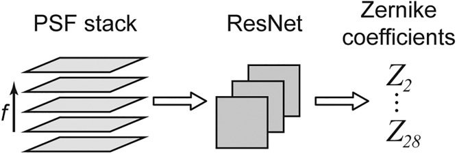
Workflow. A stack with a few images of the PSF at different focal positions f is supplied to a deep residual neural net, which processes the images and directly returns the Zernike coefficients of order 1–6 (Noll indices 2–28) that correspond to the phase information encoded in the PSF images.

FIG. 2.

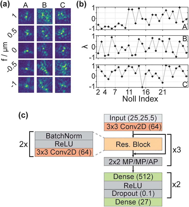
(a) Three representative PSFs (A, B, and C) at focal positions from −1 to 1 μm. (b) Zernike coefficients for the three representative PSFs shown in (a). For clarity, only Noll indices that correspond to a change in the order of the Zernike coefficients are marked along the x-axis. (c) Schematic NN architecture. The PSF stack is supplied to the NN as a 25 × 25 pixel image with five channels, corresponding to the five focal positions. After 3 × 3 2D convolution with 64 filters, three residual blocks follow, each consisting of two stacks of batch normalizations, ReLU activation, and 3 × 3 2D convolution with 64 filters. After each residual block, the output of the residual block and its respective input are added. Then, 2 × 2 pooling is performed (MaxPooling, MP, after the first two residual blocks and average pooling, AP, after the third). Finally, two fully connected layers with 512 filters follow, each with ReLU activation and a dropout layer (dropout rate = 0.1). The last layer returns the predicted Zernike coefficients.

FIG. 3.

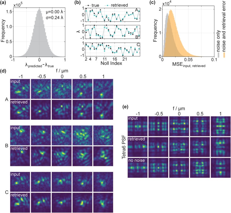
(a) Histogram of the differences in wavelength units between the retrieved and the ground truth values for all Zernike coefficients in the validation dataset. (b) Representative examples for the agreement between retrieved and ground truth Zernike coefficients for three PSFs. Notably, the prediction is accurate over the whole range of Zernike coefficients, up to the highest order. (c) Histogram of mean squared errors between input and retrieved PSFs, calculated pixelwise for each PSF slice of the 100 000 validation PSFs (orange). Input and retrieved PSFs are normalized. The high agreement between the retrieved and true Zernike coefficients translates to low MSEs. A significant fraction of the error stems from Poisson noise in the input PSFs, evident from the MSE between input PSFs without noise and input PSFs that include noise (gray histogram—“noise only” refers to the influence of Poisson noise in the input PSFs). (d) Comparison between the input PSFs at the five simulated focal positions and the PSFs generated from the retrieved Zernike coefficients, corresponding to the data plotted in (b). The agreement is very good. Note that the retrieved PSFs do not include background or Poisson noise, whereas the input PSFs to be retrieved do. (e) PR of the Tetrapod PSF with the 6 μm range (Tetra6). Retrieval results from an additional NN are included, which was trained on PSFs not including noise (no noise). Note in this case, the input PSFs do not include noise as would typically be the case for a specific phase mask design. The retrieved PSF approaches the ground truth well. As expected, the NN that was trained on PSFs without noise performs slightly better.