Detecting critical slowing down in high-dimensional epidemiological systems

Abstract

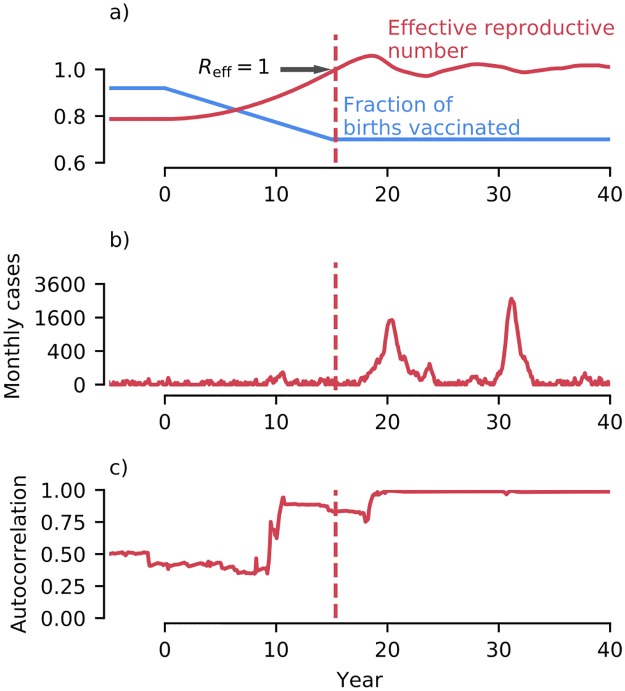
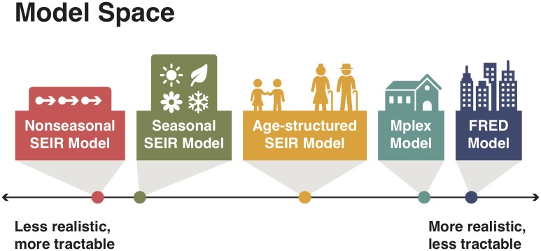
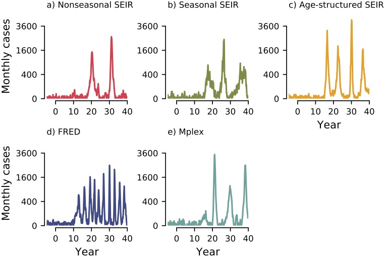
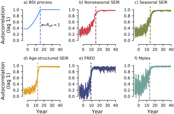
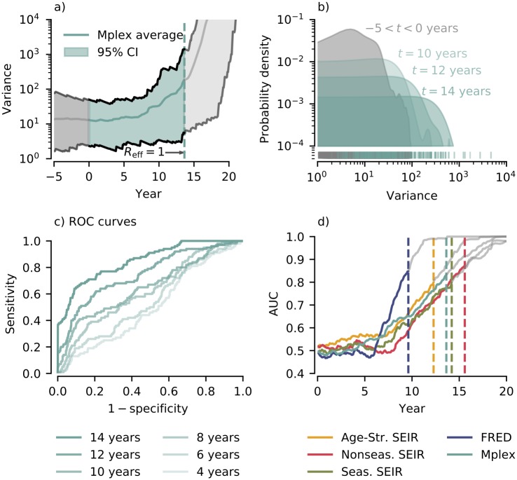
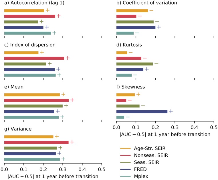
Despite medical advances, the emergence and re-emergence of infectious diseases continue to pose a public health threat. Low-dimensional epidemiological models predict that epidemic transitions are preceded by the phenomenon of critical slowing down (CSD). This has raised the possibility of anticipating disease (re-)emergence using CSD-based early-warning signals (EWS), which are statistical moments estimated from time series data. For EWS to be useful at detecting future (re-)emergence, CSD needs to be a generic (model-independent) feature of epidemiological dynamics irrespective of system complexity. Currently, it is unclear whether the predictions of CSD-derived from simple, low-dimensional systems-pertain to real systems, which are high-dimensional. To assess the generality of CSD, we carried out a simulation study of a hierarchy of models, with increasing structural complexity and dimensionality, for a measles-like infectious disease. Our five models included: i) a nonseasonal homogeneous Susceptible-Exposed-Infectious-Recovered (SEIR) model, ii) a homogeneous SEIR model with seasonality in transmission, iii) an age-structured SEIR model, iv) a multiplex network-based model (Mplex) and v) an agent-based simulator (FRED). All models were parameterised to have a herd-immunity immunization threshold of around 90% coverage, and underwent a linear decrease in vaccine uptake, from 92% to 70% over 15 years. We found evidence of CSD prior to disease re-emergence in all models. We also evaluated the performance of seven EWS: the autocorrelation, coefficient of variation, index of dispersion, kurtosis, mean, skewness, variance. Performance was scored using the Area Under the ROC Curve (AUC) statistic. The best performing EWS were the mean and variance, with AUC > 0.75 one year before the estimated transition time. These two, along with the autocorrelation and index of dispersion, are promising candidate EWS for detecting disease emergence.

Fig 1. Example simulation of disease re-emergence using the nonseasonal SEIR model.

Parameters were set to mimic transmission of a measles-like disease in a population of 10⁶ individuals, see Methods for model details and the full parameterization. a) The simulation was initialised above the herd immunity threshold, with 92% vaccine coverage. Starting in year 0, vaccine uptake of new born individuals drops linearly from 92% to 70% over 15 years. As vaccine uptake drops, R_eff increases, crossing the critical threshold R_eff = 1 shortly after 15 years. b) After the herd immunity threshold is crossed large outbreaks become possible, and endemicity is reestablished. c) Increases in early-warning signals (autocorrelation shown) precede the epidemic transition, enabling possible forewarning.

Fig 2. Representation of the trade off between tractability and realism in model construction.

Models are positioned along the axis based on the relative complexity of the model, as determined by the number of state variables (the dimensionality) and model structure (the interactions between state variables). The nonseasonal SEIR model is the simplest model, with the FRED and Mplex models being the most complex. Simpler models lend themselves to mathematical analysis, while sacrificing realism. More complex models better represent reality, at the expense of analytical tractability.

Fig 3. Example simulated time series of monthly cases for the five models (panels a–e).

Each model was parameterised to have a herd immunity threshold around 90% vaccine coverage, and experienced the same decrease in vaccine coverage over the same time span as Fig 1a. Qualitatively, we see that the effect of declining vaccine coverage is model-structure dependent. For the time series shown, the time to the first major outbreak varies between 10 years for FRED (panel d) to 18 years for the nonseasonal SEIR model (panel a).

Fig 4. Estimating of time of emergence from case reports data.

a) The Poisson transmission model assumes R_eff is a piecewise linear function of time, with a quadratic increase from $R_{\text{eff}}=R_{\text{eff}}^i$ at t = 0 to R_eff = 1 at t = Δ. The time of emergence, Δ, is estimated from the simulated data using Bayesian MCMC (see Methods). b) Final posterior density of the time of emergence. The MAP values of $\widehat{\Delta }$ for each model are listed in Table 1.

Fig 5. The autocorrelation at lag one month through time.

a) Theoretical benchmark using the BDI process, given by Eq 11. b-f) Estimates for the autocorrelation calculated for each month from the ensemble of realisations. MAP estimates of the time of emergence, $\widehat{\Delta }$, are indicated by dashed vertical lines. For all models, the autocorrelation increases as the time of emergence is approached, indicative of CSD.

Fig 6. Performance of the variance at detecting emergence.

a) Variance for the Mplex model calculated using an exponentially weighted moving window with a half life of 3 years. Mean and 95% credible interval calculated using 100 realizations. b) Test (green) and null (grey) probability densities for the variance. Probability densities found using kernel density estimation (see Methods). Null probability density calculated using all data points in the interval −5 < t < 0 years. Test probability densities shown for t = 10, 12, 14 years. c) ROC curves for the variance for the Mplex model shown for 2 year intervals. d) Area Under the ROC Curve (AUC) through time for the variance for each model. Vertical lines indicate the time of emergence.

Fig 7. Summary of the AUC values one year before the transition.

a–g) AUC values for each model for the EWS indicated in the panel. The + (−) symbols next to each bar indicate that the AUC is greater (less) than 0.5.

References

-
- Hohenberg PC, Halperin BI. Theory of dynamic critical phenomena. Reviews of Modern Physics. 1977;49(3):435 10.1103/RevModPhys.49.435 - DOI
- Bailey NTJ. The Elements of Stochastic Processes with Applications to the Natural Sciences. vol. 25 John Wiley & Sons; 1990.
- van Kampen NG. Stochastic Processes in Physics and Chemistry. North Holland; 1981.
- Strogatz SH. Nonlinear Dynamics and Chaos: With Applications to Physics, Biology, Chemistry and Engineering. Westview Press; 2001.
Publication types
MeSH terms
Grants and funding
LinkOut - more resources
Full Text Sources