The temporal structure of the inner retina at a single glance

Abstract

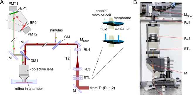
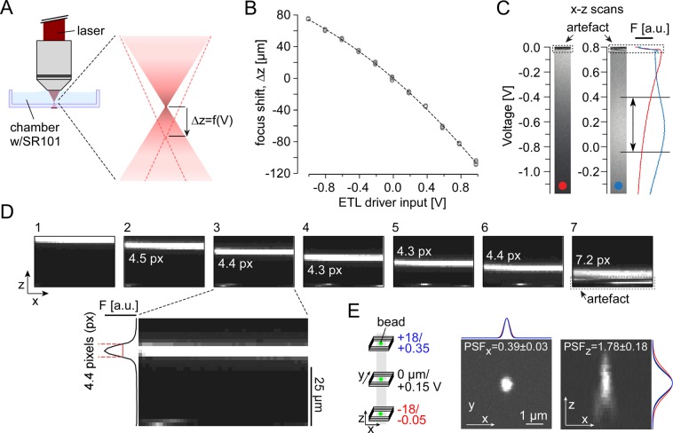
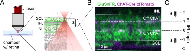
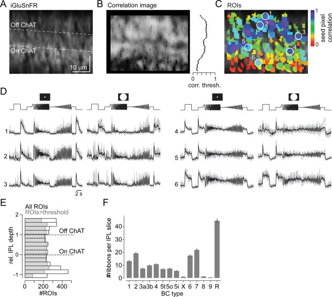
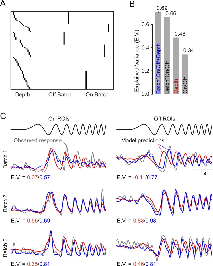
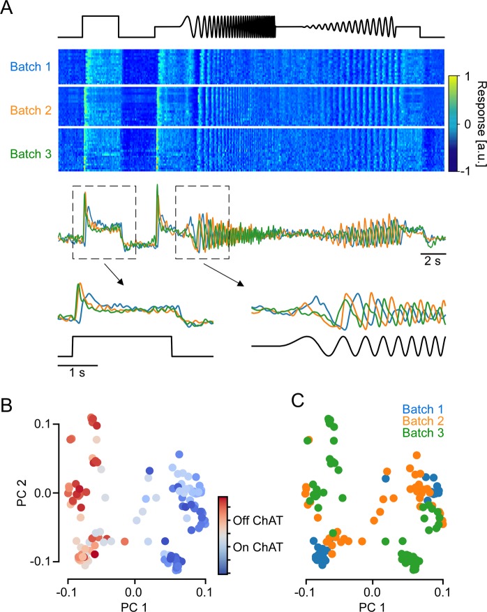
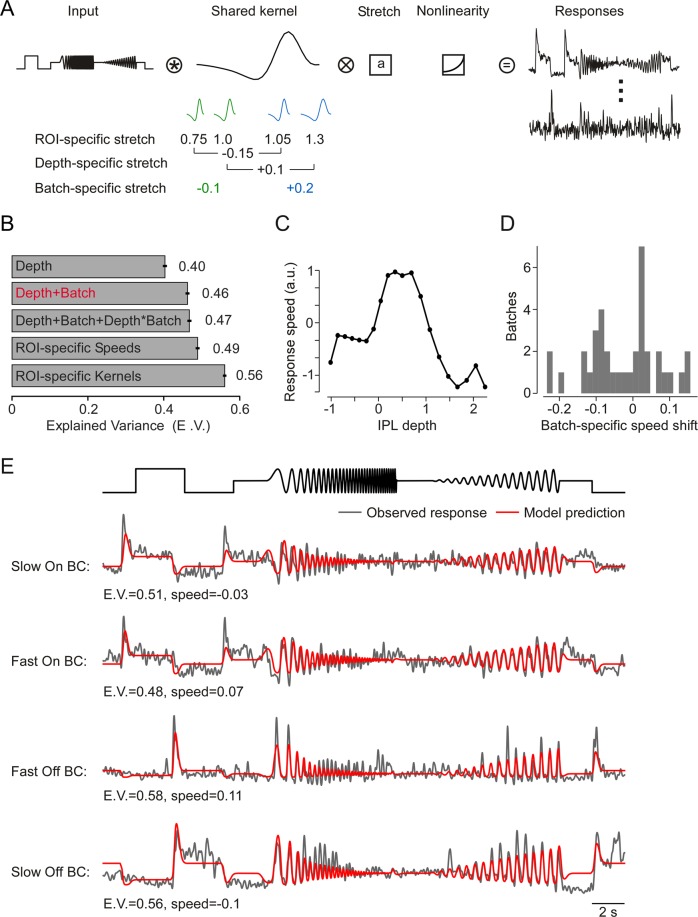
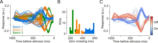
The retina decomposes visual stimuli into parallel channels that encode different features of the visual environment. Central to this computation is the synaptic processing in a dense layer of neuropil, the so-called inner plexiform layer (IPL). Here, different types of bipolar cells stratifying at distinct depths relay the excitatory feedforward drive from photoreceptors to amacrine and ganglion cells. Current experimental techniques for studying processing in the IPL do not allow imaging the entire IPL simultaneously in the intact tissue. Here, we extend a two-photon microscope with an electrically tunable lens allowing us to obtain optical vertical slices of the IPL, which provide a complete picture of the response diversity of bipolar cells at a "single glance". The nature of these axial recordings additionally allowed us to isolate and investigate batch effects, i.e. inter-experimental variations resulting in systematic differences in response speed. As a proof of principle, we developed a simple model that disentangles biological from experimental causes of variability and allowed us to recover the characteristic gradient of response speeds across the IPL with higher precision than before. Our new framework will make it possible to study the computations performed in the central synaptic layer of the retina more efficiently.

Figure 1

Overview of the two-photon (2 P) microscope equipped with an electrically tunable lens (ETL). For simplicity, most lenses and silver mirrors (M) were omitted. For parts, see Table 1. (A) Schematic diagram of the microscope’s main optical paths, with the EL-16-40-TC (Optotune) inserted before the x-y galvo scan mirrors (M_Scan). Inset: Cross section and working principle of the ETL; a voice-coil actuator generates pressure on a container, which in turn pushes optic fluid into the lens volume sealed by polymer membrane and, thereby, modulating the curvature of the lens surface. (B) Photograph of the excitation path before the scan mirrors. CM, cold mirror; DM, dichroic mirror; BP, band pass filter; PMT, GaAsP photomultiplier tube; RL, relay lens; T, telescope. Panel A adapted from Euler et al., inset adapted from Optotune website (https://www.optotune.com/).

Figure 2

Axial scan properties. (A) Illustration of the measurement configuration and the excitation laser’s focus shift (Δz) introduced by the ETL. (B) Axial position (measured with the microscope stage motor) as a function of voltage input to ETL driver (circles represent n = 5 individual measurements per voltage performed in random sequence; dashed curve represents sigmoidal fit). (C) Sulforhodamine 101 (SR101) solution in the chamber was used to measure fluorescence intensity as function of focus shift for two exemplary ETL voltage offsets; x-z scan field (left; 256 × 256 pixels, 2 ms/line; zoom_XY,Z = 1.0, 0.8) and mean fluorescence (right). Arrow indicates range (~40 µm) of near-constant fluorescence. Dotted rectangles on the top indicate artefact. (D) Axial x-z scan (64 × 40 pixels, 2 ms/line, zoom_XY,Z = 1.0, 1.0, V_Offset = 0.15 V) of a 5 μm-thin film of fluorescein solution between two coverslips (measured using the microscopes motorized stage) at different z-positions. After jumping back to the beginning of a frame, the ETL requires a few milliseconds to settle; this “settling” generates an artefact at the bottom of the frame and makes the film appear wider in frame 7 (for details, see Results). Inset: Frame 3 with intensity distribution along z-axis; for this scan configuration, the fluorescent band width was 4.4 pixels ± 0.1 (mean ± s.d. for width at half maximum, n = 5 measurements), corresponding to a pixel “height” of 1.1 µm. (E) Illustration of point spread function (PSF) measurements at three positions (−18 (red), 0 (black), 18 μm (blue)) along the z-axis (right); example images of fluorescent beads (170-nm beads, λ_{Em, Peak} = 515 nm; 256 × 256 pixels, n = 60 z-planes, Δz = 0.2 µm, zoom_XY = 8) at 0 μm, with mean Gaussian fits (n = 3 measurements/plane). PSF_x and PSF_z indicate the mean ± s.d. across the three axial planes (n = 9 measurements; see Table 3).

Figure 3

Mapping the inner plexiform layer (IPL). (A) Illustration of axial scans in the whole-mount retina of a transgenic mouse expressing tdTomato under the ChAT promotor and iGluSnFR via AAV transduction (Methods). (B) Axial x-z scan (256 × 160 pixels, 2 ms/line, zoom_XY,Z = 1.5, 0.75) with iGluSnFR expression (green) and ChAT bands (magenta). IPL borders and ChAT bands (solid and dashed lines, respectively) were defined manually (Methods). Note that the retina was flipped from (A), following the convention to show the photoreceptors pointing up. C, IPL border positions relative to ChAT bands (left; INL: 1.9 ± 0.1; GCL: −1.1 ± 0.1; n = 3/6/14 mouse/retinas/scans).

Figure 4

Glutamate imaging in the inner plexiform layer. (A) Axial x-z scan (64 × 56 pixels, 1.6 ms/line) of the inner plexiform layer (IPL) in a whole-mount wild-type mouse retina expressing iGluSnFR ubiquitously after AAV-mediated transduction. (B) Correlation image (left) and distribution of correlation thresholds across the IPL (right). (C) ROIs extracted from scan in (A), pseudo-coloured by seed pixel correlation (for details on ROI extraction, see Methods). (D) Glutamate responses to local and global chirp stimulus for exemplary ROIs encircled in (C); Off (left) and On responses (right) are shown. (E) Distribution of all ROIs (black, n = 5,379) and ROIs that passed our quality threshold (grey, n = 3,893; Methods) recorded across the IPL (n = 6/8/37 mice/retinas/scans). (F) Number of ribbon synapses from different BC types per vertical IPL slice (Methods), estimated based on available EM data.

Figure 5

Batch effect estimation using linear models. (A) Design matrix with IPL depth and batch specific predictors (example scan fields from Fig. 6). (B) Model comparison for On/Off, batch and IPL depth in a linear model fitted to the local chirp response data (same dataset as in Fig. 4A-E). Error bars indicate 2 S.E.M. (C) Example traces (grey) for first ROI of each polarity and batch shown in Fig. 6A. Predicted responses from model using IPL depth alone (red) and with an additional batch specific term (blue). E.V., Explained Variance.

Figure 6

Batch effects in axial x-z scans of the mouse inner plexiform layer (IPL). (A) Local chirp responses from ROIs located in the On sublamina of the IPL. From top: time course of chirp stimulus, heat map showing glutamate responses of ROIs from three scan fields (batches), average glutamate responses over ROIs in each batch, and magnified step and frequency responses. (B,C), Local chirp responses of ROIs in (A) projected onto their first two principal components (PCs), coloured by IPL depth (B) and batch (C).

Figure 7

Encoding model comparison. (A) Model design: the input time series of the chirp stimulus is convolved with a finite impulse response linear filter which is sign-flipped for On and Off responses and stretched by a factor that is learned for each ROI, then passed through a static nonlinearity (exponential linear unit) and weighted by each ROI to produce the predicted trace. (B) Comparison of the different speed models (Methods) learned simultaneously with the encoding model. Error bars indicate 2 S.E.M. (C) Speed as a function of IPL depth. (D) Distribution over learned batch shifts. (E) Observed (black) and predicted (red) traces for four ROIs. E.V., Explained Variance.

Figure 8

Differences in response speed between batches. (A) Learned temporal kernels for all ROIs with E.V. > 0.5. Coloured by batch (same batches as in Fig. 5). (B) Zero crossings (after first peak) for all ROIs with E.V. > 0.3. (C) All ROIs of the 2^nd batch (orange in A,B) with E.V. > 0.3, coloured by IPL depth.

References

1. Masland RH. The neuronal organization of the retina. Neuron. 2012;76:266–280. doi: 10.1016/j.neuron.2012.10.002. - DOI - PMC - PubMed
1. Wässle H. Parallel processing in the mammalian retina. Nat. Rev. Neurosci. 2004;5:747–757. doi: 10.1038/nrn1497. - DOI - PubMed
1. Euler T, Haverkamp S, Schubert T, Baden T. Retinal bipolar cells: elementary building blocks of vision. Nat. Rev. Neurosci. 2014;15:507–519. doi: 10.1038/nrn3783. - DOI - PubMed
1. Diamond JS. Inhibitory Interneurons in the Retina: Types, Circuitry, and Function. Annu. Rev. Vis. Sci. 2017;3:1–24. doi: 10.1146/annurev-vision-102016-061345. - DOI - PubMed
1. Lukasiewicz PD, Shields CR. Different combinations of GABAA and GABAC receptors confer distinct temporal properties to retinal synaptic responses. J. Neurophysiol. 1998;79:3157–3167. doi: 10.1152/jn.1998.79.6.3157. - DOI - PubMed
Publication types