The use of mixture density networks in the emulation of complex epidemiological individual-based models

Abstract

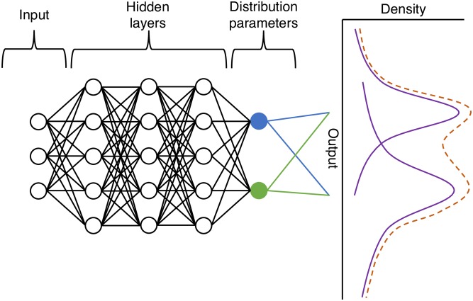
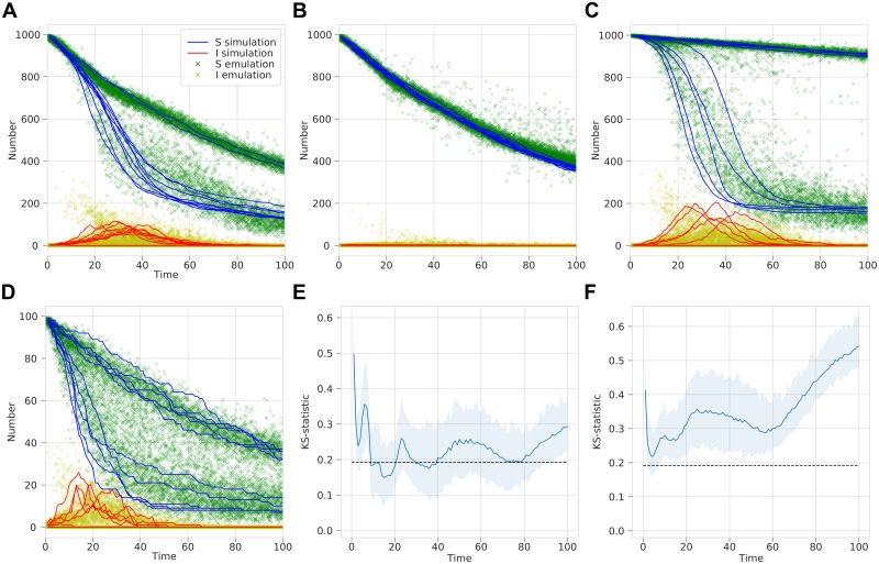
Complex, highly-computational, individual-based models are abundant in epidemiology. For epidemics such as macro-parasitic diseases, detailed modelling of human behaviour and pathogen life-cycle are required in order to produce accurate results. This can often lead to models that are computationally-expensive to analyse and perform model fitting, and often require many simulation runs in order to build up sufficient statistics. Emulation can provide a more computationally-efficient output of the individual-based model, by approximating it using a statistical model. Previous work has used Gaussian processes (GPs) in order to achieve this, but these can not deal with multi-modal, heavy-tailed, or discrete distributions. Here, we introduce the concept of a mixture density network (MDN) in its application in the emulation of epidemiological models. MDNs incorporate both a mixture model and a neural network to provide a flexible tool for emulating a variety of models and outputs. We develop an MDN emulation methodology and demonstrate its use on a number of simple models incorporating both normal, gamma and beta distribution outputs. We then explore its use on the stochastic SIR model to predict the final size distribution and infection dynamics. MDNs have the potential to faithfully reproduce multiple outputs of an individual-based model and allow for rapid analysis from a range of users. As such, an open-access library of the method has been released alongside this manuscript.

Fig 1. MDN that emulates a model with three inputs and a one-dimensional output with two mixtures.

The inputs are passed through two hidden layers, which are then passed on to the normalised neurons, which represent the parameters of a distribution and its weights e.g. the mean (shown in blue) and variance (shown in green) of a normal distribution. These parameters are used to construct a mixture of distributions (represented as a dashed line).

Fig 2. Gamma-MDN output emulating a negative binomial model.

(A) For fixed shape parameter k = 2.5, the distribution of output from MDN is shown in blue (mean = solid line, variance = shaded region), the theoretical values are shown as a black dashed line (mean = bold line, variance = normal line). (B) For fixed mean parameter m = 50, the distribution of output from MDN over a range of k values is shown in blue (mean = solid line, variance = shaded region), the theoretical values are shown as a black dashed line (mean = bold line, variance = normal line). (C) Corresponding two-sample K–S statistic where sample of 100 points are drawn from a negative binomial and the MDN over a range of m values. 100 replicates are used to estimate a mean K–S statistic and a 95% range. The dashed line represents significance at α = 0.05, with values less than this indicating that the two samples do not differ significantly. (D) Example empirical CDFs drawn from 100 samples of MDN with inputs m = 50 and k = 2.5. 1,000 empirical CDFs are shown as black transparent lines and true CDF is shown as a blue solid line.

Fig 3. Binomial-MDN output emulating the final size distribution of a stochastic SIR model.

(A) For random uniform sampling over β and γ a sample of the output from MDN across values for the basic reproductive number R₀ = β/γ are shown in blue and the directly simulated values are shown in red. (B) Corresponding two-sample K–S statistic where sample of 100 points are drawn from a negative binomial and the MDN over a range of R₀ values. 100 replicates are used to estimate a mean K–S statistic and a 95% range. Dashed line represent significance at α = 0.05, with values less indicating the two samples do not differ significantly. (C) The percentage of 1,000 realisations of the stochastic SIR model with final size greater than 100 is shown in black with dashed line showing a 95% range. Emulated results are shown by the blue line with a 95% range. (D) Example empirical CDFs drawn from 100 samples of MDN with inputs β = 0.4 and γ = 0.2. 1,000 empirical CDF are shown as black transparent lines and true CDF is shown as a blue solid line.

Fig 4. Beta-MDN output emulating the infection dynamics with time for a stochastic SIR model.

(A–D) A comparison of simulation results with sampled MDN output for fixed γ = 0.2 and N = 1, 000 and different β values that give the following R₀ values: (A) R₀ = 0.5, (B) R₀ = 1.0, (C) R₀ = 2.0, and (D) R₀ = 5.0. (E–F) Two-sample K–S statistic where sample of 100 points are drawn from a negative binomial and the MDN over a range of time t values. 100 replicates are used to estimate a mean K–S statistic and a 95% range. Dashed line represent significance at α = 0.05, with values less indicating the two samples do not differ significantly. Tests are for (E) number of susceptible people and (F) number of infected people.

Fig 5. Beta-MDN output emulating the infection dynamics with time for a stochastic SIR model.

(A–D) A comparison of simulation results with sampled MDN output for fixed γ = 0.2 and different β, δ and N values such that (A) R₀ = 2.0, δ = 0.01 and N = 1, 000, (B) R₀ = 1.0, δ = 0.01 and N = 1, 000, (C) R₀ = 2.0, δ = 0.001 and N = 1, 000, (D) R₀ = 2.0, δ = 0.01 and N = 100. (E–F) Two-sample K–S statistic where sample of 100 points are drawn from a negative binomial and the MDN over a range of time t values. 100 replicates are used to estimate a mean K–S statistic and a 95% range. Dashed line represent significance at α = 0.05, with values less indicating the two samples do not differ significantly. Tests are for (E) number of susceptible people and (F) number of infected people.

References

-
- Keeling MJ, Rohani P. Modeling infectious diseases in humans and animals. Princeton University Press; 2011.
- May RM. Togetherness among schistosomes: its effects on the dynamics of the infection. Mathematical Biosciences. 1977;35(3-4):301–343. 10.1016/0025-5564(77)90030-X - DOI
- Irvine MA, Reimer LJ, Njenga SM, Gunawardena S, Kelly-Hope L, Bockarie M, et al. Modelling strategies to break transmission of lymphatic filariasis-aggregation, adherence and vector competence greatly alter elimination. Parasites & Vectors. 2015;8(1):547 10.1186/s13071-015-1152-3 - DOI - PMC - PubMed
Publication types
MeSH terms
Grants and funding
LinkOut - more resources
Full Text Sources
Medical
Research Materials