Improved detection of differentially represented DNA barcodes for high-throughput clonal phenomics

Abstract

Cellular DNA barcoding has become a popular approach to study heterogeneity of cell populations and to identify clones with differential response to cellular stimuli. However, there is a lack of reliable methods for statistical inference of differentially responding clones. Here, we used mixtures of DNA-barcoded cell pools to generate a realistic benchmark read count dataset for modelling a range of outcomes of clone-tracing experiments. By accounting for the statistical properties intrinsic to the DNA barcode read count data, we implemented an improved algorithm that results in a significantly lower false-positive rate, compared to current RNA-seq data analysis algorithms, especially when detecting differentially responding clones in experiments with strong selection pressure. Building on the reliable statistical methodology, we illustrate how multidimensional phenotypic profiling enables one to deconvolute phenotypically distinct clonal subpopulations within a cancer cell line. The mixture control dataset and our analysis results provide a foundation for benchmarking and improving algorithms for clone-tracing experiments.

Keywords: DNA barcoding; clone tracing; fate mapping; lineage tracing; phenomics.

Figure 1. An overview of the experimental setup for the benchmark dataset generation

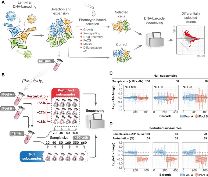
1. A schematic presentation of a typical clone‐tracing experiment (see text for description).

2. To generate the benchmark barcode count datasets, we performed two independent high‐complexity DNA barcoding experiments on Mia‐PaCa‐II and OVCAR5 cell lines (see Materials and Methods for details). In each experiment, cells were collected after selection and expansion step (Fig 1A) to produce two cell pools (Pool A and Pool B). Cells in each pool were counted and mixed in a 50/50 ratio to produce “AB mix”. The AB mix was then sampled in various extents in two replicas to produce so‐called null samples with different numbers of cells (20 × 10³, 40 × 10³, 80 × 10³, 160 × 10³, 330 × 10³, 660 × 10³), but with the same expected representation of each barcode. Perturbed samples were generated by taking either 20, 40, 80 or 160 thousand cells from the AB mix, and adding an indicated percentages of cells from the Pool A (e.g. for sample with 160 × 10³ cells and perturbation degree of 35%, we added 160 × 10³ × 0.35 = 56 × 10³ cells from the Pool A). The number of replicas for each sample is indicated in circles next to the tube icon.

3. Barcode representation fold changes (log₂) in the null samples of the indicated sizes (number of cells sampled from the AB mix), relative to the mean of two Null‐660 replicas. Barcodes are ordered according to their size in the Null‐660 samples. Pool A barcodes are sorted in decreasing order, and Pool B barcodes are ordered in increasing order. Boxes represent interquartile ranges for each group of 53 observations. Whiskers indicate upper and lower quartiles. Central line corresponds to the median value.

4. Same data as in (C) but for the perturbed samples. Dotted lines indicate the expected barcode fold changes calculated using formula: (cells from pool A/total number of cells)/0.5, for the Pool A barcodes, and similarly for the Pool B barcodes. Data representation is the same as in (C).

Figure 2. Sampling size affects the statistical properties and accuracy of DRB detection

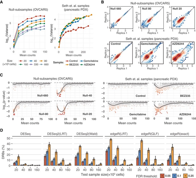
1. Mean–variance plots for the benchmark OVCAR5 null samples and pancreatic cancer patient‐derived xenograft (PDX) samples (Seth et al, 2019). Local variance was calculated by averaging a tagwise variance over the mean counts using a 20 read‐count window.

2. Scatterplots of median‐normalized read counts (log₁₀) of OVCAR5 null samples and pancreatic PDX samples (Seth et al, 2019).

3. Local goodness‐of‐fit testing for negative binomial distribution where the distribution parameters were estimated using maximum‐likelihood estimator (MLE). Two‐sample Cramer–von Mises test was used to compare the observed and simulated negative binomial random variables. Statistical significance was determined using Monte Carlo bootstrap method, where a small empirical P‐value indicates strong deviation from the negative binomial distribution.

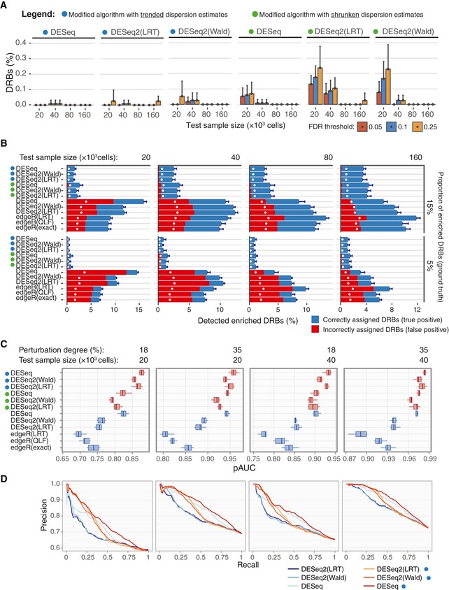
4. The proportion of differentially represented barcodes (DRBs) identified in the OVCAR5 null samples with various versions of RNA‐seq analysis algorithms. Two replicas of the null samples of indicated sizes (x‐axis) were tested for DRBs against a control group of 4 null samples (two Null‐660 samples and two Null‐330 samples). The bars represent the average proportion of DRBs identified with the algorithms, calculated over threefold bootstrap runs (mean of the 10 resamples with replacement) under the indicted false discovery rates (FDRs). The version with unadjusted P‐values is shown in Appendix Fig S1A for comparison. Error bars, SD; LRT, likelihood ratio test; Wald, Wald test; QLF, quasi‐likelihood F‐test; and exact, implementation of exact test proposed by Robinson and Smyth (Robinson & Smyth, 2008), as implemented in the original algorithms.

Figure EV1. Clone size characteristics of the benchmark datasets

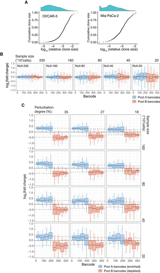
1. Cumulative distributions of clone sizes in OVCAR‐5 null‐660 sample (left) and Mia‐Paca‐2 null‐40 sample (right).

2. Barcode representation fold changes (log₂) for the null samples of the indicated sizes (number of cells subsampled from the AB mix) relative to the mean of two Null‐660 replicas. Barcodes are ordered according to the size in the Null‐660 subsamples. Pool A barcodes are sorted in the descending order, and Pool B barcodes are ordered in the ascending order. Boxes represent interquartile ranges (25 to 75 percentile) for each group of 53 observations. Whiskers indicate upper and lower quartiles. Central line corresponds to the median value.

3. Same as Fig EV1B but for the perturbed subsamples. Dotted lines indicates the expected barcode fold changes calculated using formula: (cells from pool A/total number of cells)/0.5, for the Pool A barcodes, and formula: (cells from pool B/total number of cells)/0.5, for the Pool B barcodes. Data representation is the same as in (B).

Figure EV2. Sampling size affects statistical properties and accuracy of DRB calling.

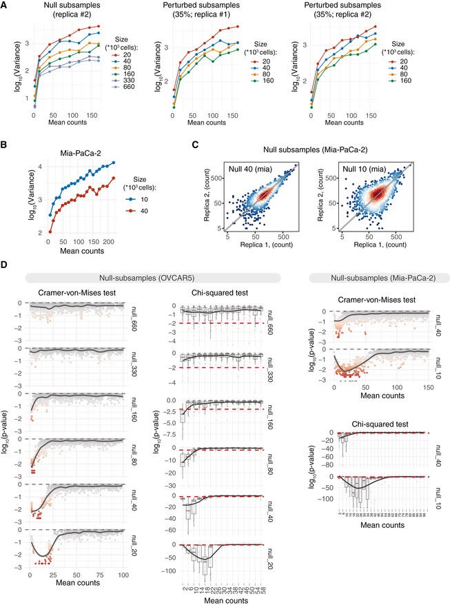
1. Mean–variance plots for the benchmark OVCAR5 null subsamples (replica#2) and perturbed subsamples (35% perturbation degree; replicas #1 and #2). Local variance was calculated by averaging a tagwise variance over the mean counts using a 20 read‐count window. Mean counts were estimated using all the null or perturbed samples, respectively.

2. Mean–variance plots for Mia‐PaCa‐2 null subsamples. Barcode read counts were median‐normalized. Local variance was calculated by averaging a tagwise variance over the mean counts using a 20 read‐count window.

3. Scatter plots of median‐normalized read counts of Mia‐PaCa‐2 null subsamples.

4. Local negative binomial goodness of fit was estimated using chi‐squared test or Cramer–von Mises test. Dispersion parameter of the negative binomial model was estimated locally over the window of 3 read counts using maximum‐likelihood estimator. P‐value of the chi‐squared test statistics was estimated using fitdistrplus::gofstat() function. P‐values of the Cramer–von Mises test were calculated by Monte Carlo bootstrap method as implemented in RVAideMemoire::cramer.test.

Figure 3. Comparison of the algorithms’ performance

Circles left to the algorithms’ names indicate the modified algorithms.

1. Barplots of the percentage of DRBs identified by the modified algorithms in the OVCAR5 null samples, calculated over threefold bootstrap runs (10 resamples with replacement) using the same design as in Fig 2D. Error bars, SD.

2. The performance of the original and modified algorithms for detection of enriched barcodes in the perturbed samples. Two replicas of the sample with perturbation degree of 35%, indicated size (top) and enriched proportions (right), were tested against four null samples (two replicas of Null‐660 samples and two replicas of Null‐330 samples). The bars represent the average percentage of the barcodes detected as enriched DRBs (fold change > 0; FDR < 0.25) by the indicated algorithm, calculated over threefold bootstrap runs (10 resamples with replacement). Correctly assigned barcodes (classified according to the ground truth) are marked in blue and incorrectly detected barcodes (not classified according to the ground truth) are marked in red (see Fig EV3 for the results in the samples with other perturbation degrees and proportions of enriched barcodes). White circles mark the percentage of barcodes corresponding to the nominal FDR level. Error bars, SD.

3. The standardized partial area under the precision‐recall curve (pAUC), calculated using intervals of [0,1] for precision and [0,X] for recall, where X is the mean recall value at FDR = 0.25 for a given sample over all the tested algorithms. The panel shows the pAUC for perturbed samples of indicted size and perturbation degree with enriched barcode proportion of 0.5 (see Appendix Figs S5 and S6 for pAUCs and precision‐recall curves for other sample sizes, perturbation degrees and proportions of enriched barcodes). For calculating the precision and recall metrics, we ranked the barcodes according to their unadjusted P‐values as classification scores, where the positive class was defined as correctly detected barcodes (correctly assigned to either enriched or depleted group; see Materials and Methods for details). A total of 10 threefold bootstrap runs with replacement were performed. Boxes represent interquartile ranges (25 to 75 percentile). Whiskers indicate upper and lower quartiles. Central line corresponds to the median value.

4. The full precision‐recall curves for the corresponding sample sizes and perturbation degrees as in (C), with enriched barcode proportion of 0.5. For clarity, the modified algorithms with shrunken dispersion estimates are not shown here.

Figure EV3. Comparison of the algorithm’ performance on the perturbed subsamples

1. A–C

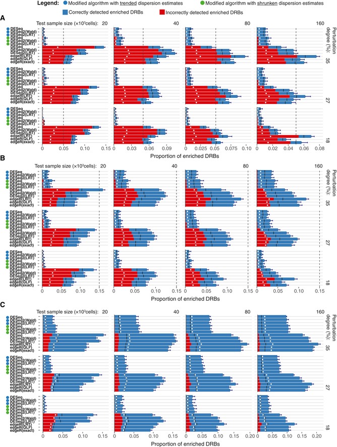
   Circles left to the algorithms’ names indicate the modified algorithms. Two replicas of the perturbed subsamples of indicated sample size (top), perturbation degree (right) and enriched barcode ratios of 0.05 (A), 0.15 (B) and 0.5 (C) were tested for DRBs against four control samples (two Null‐660 samples and two Null‐330 samples). Bars represent the average proportion of DRBs classified as enriched (fold change > 0) under the FDR threshold of 0.25, calculated over threefold bootstrap runs (10 resamples with replacement). Red bars indicate the average fraction of false positives (incorrectly assigned to the enriched group). Black lines indicate the “random” FDR—the average fraction of false discoveries observed when P‐values were randomly permuted over the barcodes. White points indicate the nominal FDR threshold of 0.25. Dashed vertical lines indicate the total proportion of enriched barcodes. Error bars, SD.

Figure EV4. Design of the carboplatin phenotyping experiments and the reproducibility of the DRB detection in the reference sample

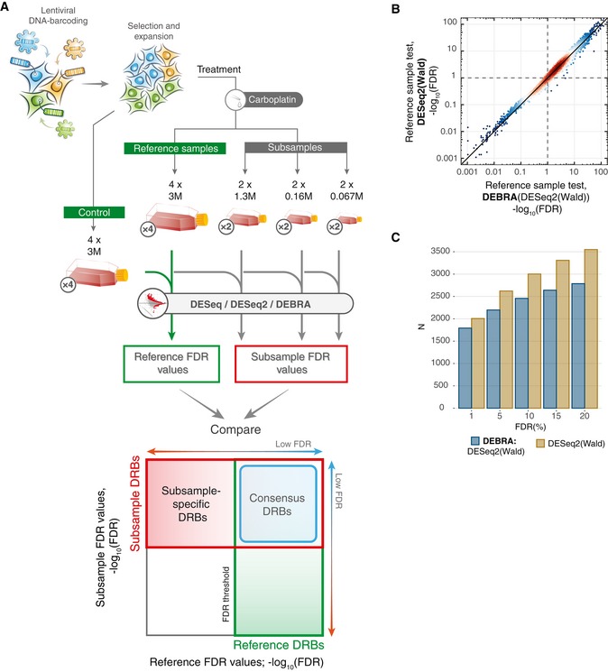
1. Overview of the experimental design for the benchmark carboplatin phenotyping experiment. Cells were barcoded and expanded to achieve the average number of 1,000 cells per clone (see Materials and Methods). Next, the cells were divided into control samples (4 × 3 M), reference samples (4 × 3 M) and subsamples (2 × 1.33 M; 2 × 0.16 M and 2 × 0.067 M). Reference and subsamples were treated with carboplatin (IC50; 7 μM) for 4 days and then allowed to re‐grow for 4 days. Barcode read counts from treated samples were tested against control samples with modified and non‐modified algorithms. Obtained FDR values were then compared to detect the consensus DRBs (consistently detected in both subsamples and reference samples; outlined with blue square) and subsample‐specific DRBs (detected only in the subsample but not in the reference sample). The number of replicas for each sample is indicated in circles next to the tube icon.

2. Scatter plot of the FDR values detected with the DEBRA‐modified DESeq2(Wald) versus original DESeq2(Wald) algorithms.

3. The number of DRBs identified with different FDR thresholds using the DEBRA‐modified DESeq2(Wald) or original DESeq2(Wald).

Figure 4. Comparison of algorithm performance for carboplatin response phenotyping

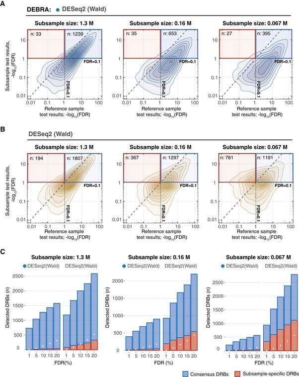
1. A, B

   Density plots of FDR values estimated in reference sample (x‐axis), plotted against corresponding FDR values in subsamples of different sizes (y‐axis), where FDR was estimated with (A) DEBRA‐modified DESeq2(Wald) or (B) original DESeq2(Wald). Blue square indicates the region where barcodes have FDR values lower than the set threshold of 0.1 in both reference and subsamples (consensus DRBs). Red square outlines the region where the barcodes are detected as significant only in the test subsample (subsample‐specific DRBs), with the total number of detected DRBs (n) indicated in the top‐left corner.

2. C

   The number of DRBs with FDR lower than a pre‐selected threshold (x‐axis), detected with the DEBRA‐modified DESeq2(Wald) (indicated by the blue circle) and original DESeq2(Wald) algorithms in subsamples of indicated sizes (top). Blue bars indicate the number of barcodes detected as significant both in reference and in subsample (consensus DRBs), and red bars indicate the number of DRBs detected only in subsample but not in reference sample. White circles mark the percentage of barcodes corresponding to the nominal FDR level.

Figure 5. Multidimensional phenotypic profiling approach

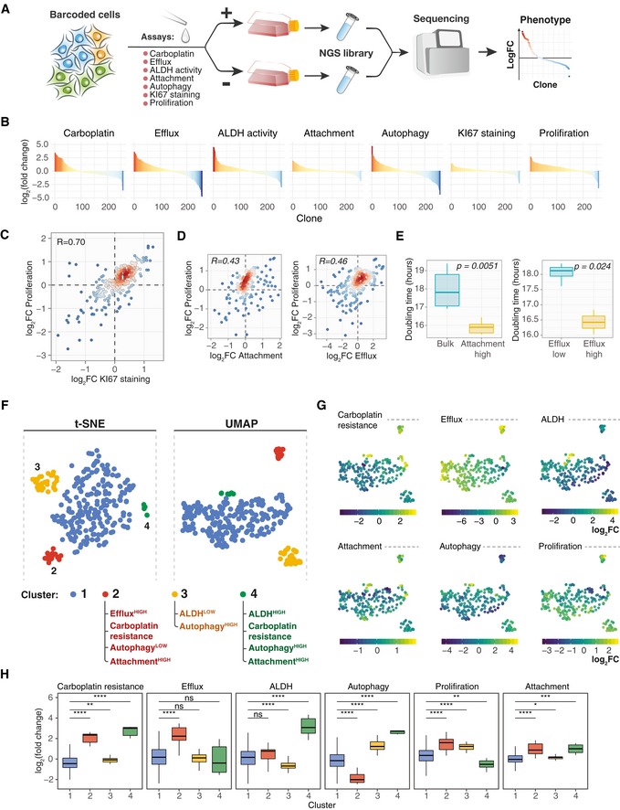
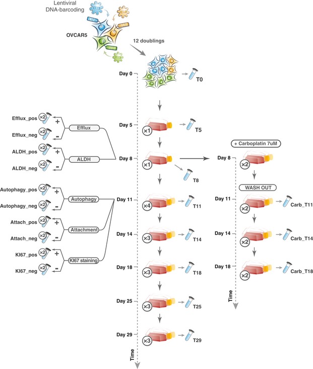
1. A schematic presentation of the experimental workflow for barcoding‐based high‐throughput multidimensional clonal lineage phenomics approach. Cells were barcoded and expanded to achieve reasonable representation of cells per barcode (e.g. 500–4,000). Next, the population was divided into multiple samples and selection pressure was applied to each sample. Cells passing selection conditions were collected and used to prepare a NGS library. In the present study, we measured clone‐specific fold changes in barcode representation in the following assays: carboplatin response (7 μM carboplatin for 3 days followed by 7 days re‐growth), autophagy measured by autolysosomes load (FACS; Thomé et al, 2016), ALDH activity, activity of efflux pumps, proliferation (7 days), 12 h of attachment assay in FBS‐free media (attached and non‐attached cells were collected) and KI67 staining.

2. Barcode representation fold changes in response to the indicated selection pressure for the clones with mean normalized read counts larger than 70.

3. Scatterplot of fold change in the barcode representation after 7 days of growth versus fold change in representation between KI67^HIGH population and control. Each point represents a clone with colour indicating the local density of points. Displayed are only clones with counts larger than 70. R, Pearson correlation coefficient.

4. Scatterplot of fold changes in clone abundances after attachment in FBS‐free condition and 7 days of growth (left), or upon sorting by efficacy of fluorescent dye efflux and 7 days of growth (right), as described in Materials and Methods.

5. The average doubling time of the cell subpopulations separated by their attachment to substrate in FBS‐free conditions (left; n = 6 biological replicates for each group) or sorted by their efficacy to efflux fluorescent dye (right; n = 3 biological replicates for Efflux^HIGH and n = 6 biological replicates for Efflux^LOW). P‐values are from Wilcoxon test. Boxes represent interquartile ranges. Whiskers indicate upper and lower quartiles. Central line corresponds to the median value.

6. t‐SNE and UMAP projections of the OVCAR5 clonal phenotypic profiles, each point represents a clone coloured according to the manually gated clusters based on the t‐SNE projection. The clones with read counts of more than 70 were used for the statistical analysis.

7. UMAP projections of the OVCAR5 clonal phenotypic profiles. The clones are colour‐coded according to the manifestation of the phenotype, calculated as log₂ ratio of barcode fractions between (1) positively and negatively selected populations after ALDH, attachment, efflux capacity or autophagy assays; (2) treated and untreated samples for carboplatin treatment assay; or (3) day 8 and day 1 time points for proliferation assay.

8. The distribution of log₂ fold changes by clusters (n = 201, 19, 31, 7 for clusters 1–4, correspondingly) in barcode representations upon selection for the indicated phenotypes. *P < 0.05; **P < 0.01; ***P < 0.001; ****P < 0.0001; ns, non‐significant, based on Wilcoxon test. Boxes represent interquartile ranges. Whiskers indicate upper and lower quartiles. Central line corresponds to the median value.

Figure EV5. A schematic representation of OVCAR5 clonal phenotypic profiling experiment

In the proliferation assay, 3 million cells were plated in each passage, and at day 8, the population was split into 4 replicas. The tube image indicates that the sample was collected for sequencing. Sample name as used in the read count table (Dataset EV4) is marked next to the tube images. The number of replicas is indicated in the circles next to the flask/tube icons.

Figure EV6. Barcode fraction fold changes for OVCAR5 single‐clone phenotypes

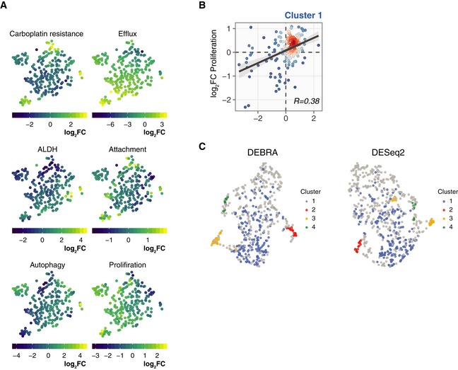
1. t‐SNE projections of the OVCAR5 clonal phenotypic profiles. The clones are colour‐coded according to the manifestation of the phenotype, calculated as log₂ ratio of barcode counts between (1) positively and negatively selected populations after ALDH, attachment, efflux capacity or autophagy assays; (2) treated and untreated samples (T14) for carboplatin treatment assay; or (3) day 8 and day 1 time points for proliferation assay.

2. Scatter plot of barcode fraction fold changes in OVCAR5 cells in response to carboplatin treatment and after 7 days of growth assay for cluster 1 (Bulk; see Fig 5F).

3. UMAP projections of the OVCAR5 clonal phenotypic profiles for clones selected according to the FDR level as determined by the DEBRA (left) or DESeq2 (right). The barcode was selected for the analysis if the minimum FDR value from the carboplatin, ALDH and efflux assays was less than 0.1. The clones are colour‐coded according to clusters as defined at Fig 5F.