Environmental remodeling of human gut microbiota and antibiotic resistome in livestock farms

Abstract

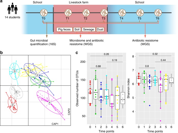
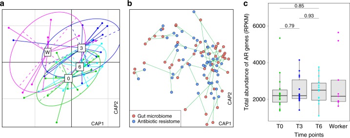
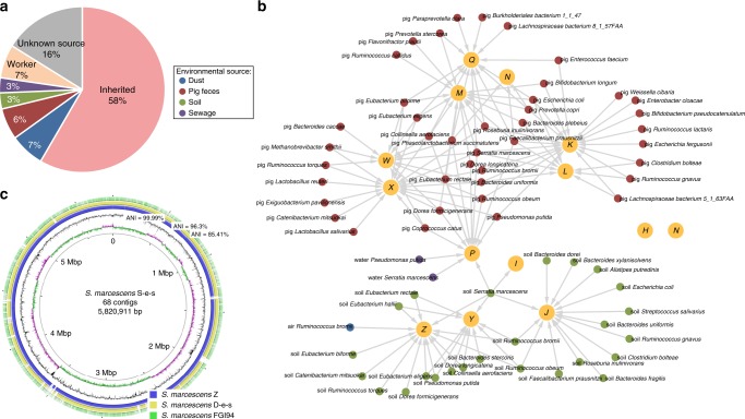
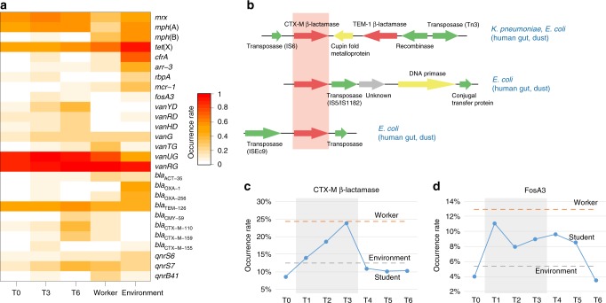
Anthropogenic environments have been implicated in enrichment and exchange of antibiotic resistance genes and bacteria. Here we study the impact of confined and controlled swine farm environments on temporal changes in the gut microbiome and resistome of veterinary students with occupational exposure for 3 months. By analyzing 16S rRNA and whole metagenome shotgun sequencing data in tandem with culture-based methods, we show that farm exposure shapes the gut microbiome of students, resulting in enrichment of potentially pathogenic taxa and antimicrobial resistance genes. Comparison of students' gut microbiomes and resistomes to farm workers' and environmental samples revealed extensive sharing of resistance genes and bacteria following exposure and after three months of their visit. Notably, antibiotic resistance genes were found in similar genetic contexts in student samples and farm environmental samples. Dynamic Bayesian network modeling predicted that the observed changes partially reverse over a 4-6 month period. Our results indicate that acute changes in a human's living environment can persistently shape their gut microbiota and antibiotic resistome.

Fig. 1. Change in the human gut microbiota following environmental conversion.

a Overview of the study design. Fourteen veterinary students’ fecal samples were collected at seven time points: T0, 1–2 weeks before work on the swine farm; T1–T3, while living and working at the swine farm; T4–T6, after returning to the university. b Distance-based redundancy analysis (dbRDA) revealed gut microbiota dysbiosis during the students’ swine farm stays, which partially recovered after leaving the farm. dbRDA of Bray–Curtis distances between operational taxonomic units (OTUs, based on 16S sequences) in samples at all-time points is shown at the first two constrained principal coordinates (CAP1 1.8% variance explained, CAP2 1.3% variance explained). Lines connect samples from the same time point, and colored circles indicate the samples near the center of gravity for each time point. The results depicted here are cumulative of the samples from three swine farms. c Change in the within-sample microbial diversity (observed number of OTUs and Shannon diversity index) of samples at seven different time points. Boxes show the distribution of students’ samples (n = 14 biologically independent samples per timepoint) (boxes show medians/quartiles; error bars extend to the most extreme values within 1.5 interquartile ranges). P > 0.05 by Student’s t-tests (paired two-sided test between the students’ samples at time points 0, 3, and 6). P-values are multiple hypothesis test corrected using Benjamini–Hochberg (FDR) correction. Underlying data are provided in the Source Data file.

Fig. 2. Change in the gut antibiotic resistomes following environmental exposure.

a Distance-based redundancy analysis (dbRDA) plot of the gut antibiotic resistomes of students’ samples at time points 0 (red), 3 (green) and 6 (blue), and workers’ samples. Lines connect samples from the same time point, and colored circles indicate the samples near the center of gravity for each time point. The first two constrained principal coordinates are shown (CAP1 2.8% variance explained, CAP2 1.6% variance explained). b Procrustes analysis connecting the microbiomes and resistomes of gut microbiota. c total abundance of the antibiotic resistance genes in students’ samples at time points 0, 3, and 6, and workers’ samples. Box plots show the distribution of students’ samples (n = 14 biologically independent samples per timepoint) (boxes show medians/quartiles; error bars extend to the most extreme values within 1.5 interquartile ranges). P > 0.05; Student’s t-tests (paired two-sided test between the students’ samples at time points 0, 3, and 6). P-values are multiple hypothesis test corrected using Benjamini–Hochberg (FDR) correction. Underlying data are provided in the Source Data file.

Fig. 3. Transmission of microbes and antibiotic resistance genes from swine farm environments.

a Origin of the genes observed in the students’ gut microbiomes during their stay on the swine farms (time point 3). The majority of the genes did not change (58%), but a large number of the newly observed genes were also identified in various swine farm habitats, such as the environment (19%, including dust, pig feces, soil, and sewage) and the workers’ gut microbiota (7%). b Species transmission network from the swine farm environment to the human gut. Larger nodes depict the students (student ID is displayed in the center of each node). Smaller nodes depict transmitted species, color-coded according to environmental types. Connecting arrows represent the transmission events. c Circular representation of the S. marcescens S-e-s draft genome (assembled from a soil sample from swine farm S) and comparison to other genomes. The inner three circles represent the genome scale, G + C skew and G + C content of the S-e-s draft genome. The outer three circles show the portions of the S-e-s genomic region that have close orthologs in other draft genomes: S. marcescens Z (blue, from one student who inherited S-e-s), S. marcescens D-e-s (yellow, from the soil sample taken from swine farm D) and S. marcescens FGI94 (green, the most homologous genome from the NCBI database). High ANI (99.9%) between S. marcescens S-e-s and Z confirmed the inheritance relationship between them. Underlying data are provided in the Source Data file.

Fig. 4. Accumulation of important antibiotic resistance genes in the human gut.

a Occurrence of the important antibiotic resistance genes in the microbiota of the students, the swine farm workers and the environment. Only important antibiotic resistance genes that were enriched in students’ gut antibiotic resistomes during their swine farm stays (time point T3) are shown. The occurrence rates of antibiotic resistance genes in each group are represented by color shading. b Representative alignment of three contigs encoding a CTX-M β-lactamase with 99% nucleotide identity. The taxonomic assignments of the contigs are indicated on the right, and source metagenomic libraries are indicated inside the parenthesis. c and d Changes in resistance detection rate of the bla_CTX-M gene c and fosA3 gene d among 1851 E. coli strains from students (blue), farm workers, and environment during the students’ swine farm residence period. The dotted lines for worker and environmental samples are the average occurrence rate of resistance genes in E. coli strains from farm workers (orange) and environment (gray) in T1, T2, and T3. Underlying data are provided in the Source Data file.

Fig. 5. Predicting students’ gut microbiotas in the next 3 months using a dynamic Bayesian network model.

DbRDA of the Bray–Curtis PCoA of the unweighted UniFrac distances between the gut microbiota in samples at the seven time points tested and three predicted future time points. Display is based on sample scores on the primary constrained axis (CAP1, 2.2% variance explained) and primary multidimensional scaling (MDS1, 20% variance explained). Lines connect samples taken at the same time point, and colored circles indicate the samples near the center of gravity for each time point. Below and left boxplots show the sample scores in CAP1 and MDS1 (boxes show medians/quartiles; error bars extend to the most extreme values within 1.5 interquartile ranges). Coding: 0, baseline; 1–3, during the swine farm stay; 4–6, 3 months after leaving the farm; 7–9, predicted time points over 3 months in the future (n = 14 biologically independent samples per timepoint for 0–6 and n = 14 predicted points per timepoint for 7–9). *P < 0.05; **P < 0.01; ***P < 0.001; NS, not significant; Student’s t-test (paired two-sided test between the students’ samples at time point T0 versus time points T3, T6, T7, T8, and T9). Underlying data are provided in the Source Data file.

References

1. Lynch SV, Pedersen O. The human intestinal microbiome in health and disease. N. Engl. J. Med. 2016;375:2369–2379. doi: 10.1056/NEJMra1600266. - DOI - PubMed
1. Donaldson GP, Lee SM, Mazmanian SK. Gut biogeography of the bacterial microbiota. Nat. Rev. Microbiol. 2016;14:20–32. doi: 10.1038/nrmicro3552. - DOI - PMC - PubMed
1. Caporaso JG, et al. Moving pictures of the human microbiome. Genome Biol. 2011;12:R50. doi: 10.1186/gb-2011-12-5-r50. - DOI - PMC - PubMed
1. Mehta RS, et al. Stability of the human faecal microbiome in a cohort of adult men. Nat. Microbiol. 2018;3:347–355. doi: 10.1038/s41564-017-0096-0. - DOI - PMC - PubMed
1. Faith JJ, et al. The long-term stability of the human gut microbiota. Science. 2013;341:1237439. doi: 10.1126/science.1237439. - DOI - PMC - PubMed
Publication types