. 2020 Aug 1:216:116760.
doi: 10.1016/j.neuroimage.2020.116760. Epub 2020 Mar 19.

Multiple testing correction over contrasts for brain imaging

Affiliations

Multiple testing correction over contrasts for brain imaging

Bianca A V Alberton et al. Neuroimage. .

Abstract

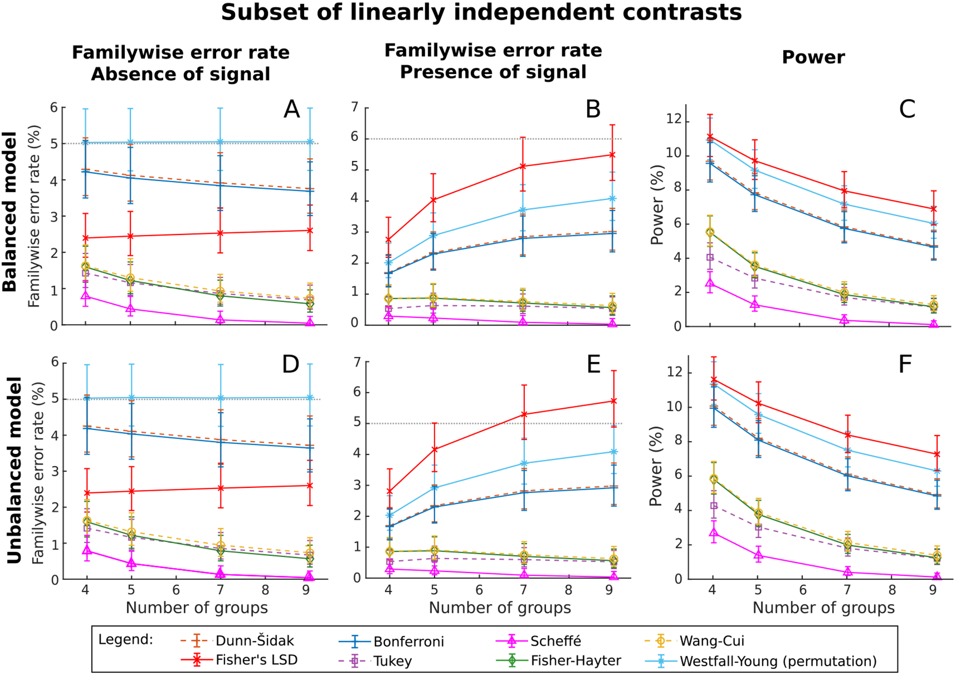
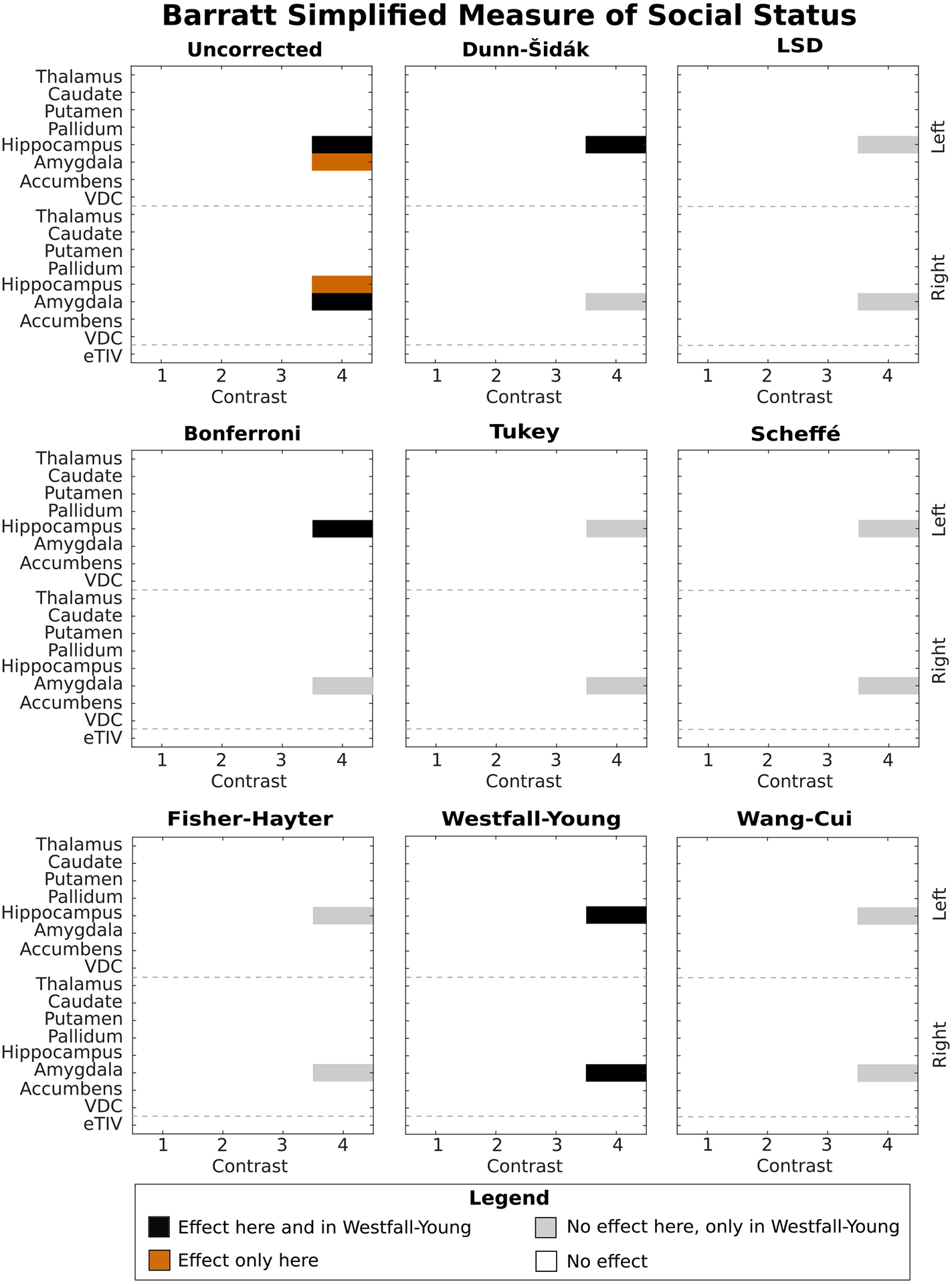
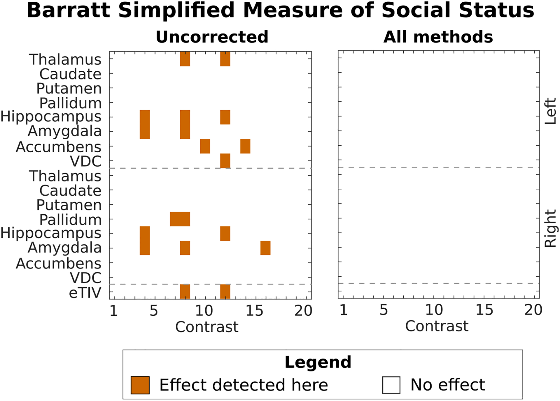
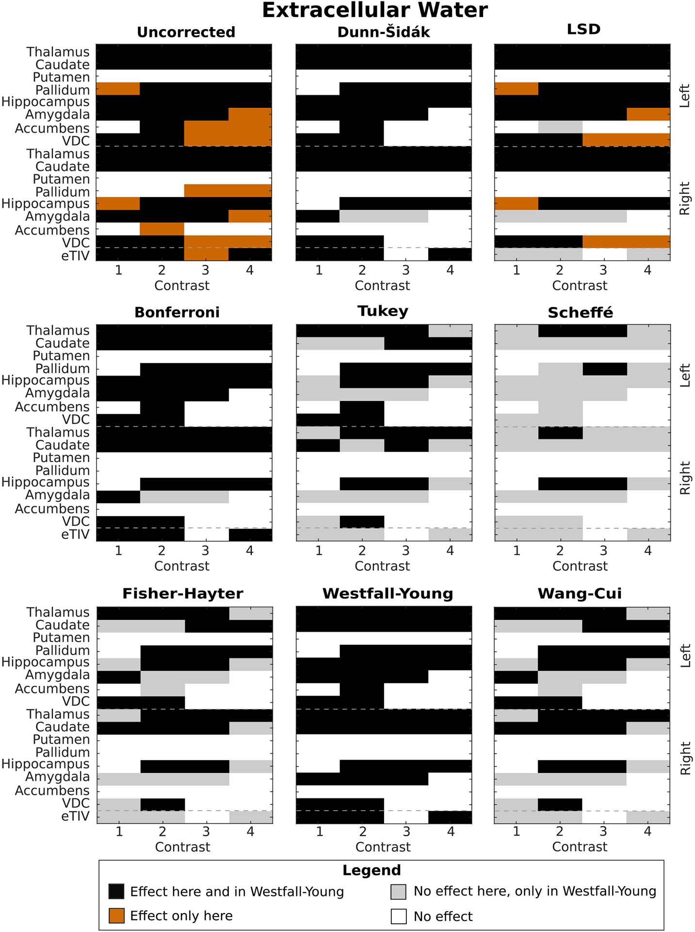
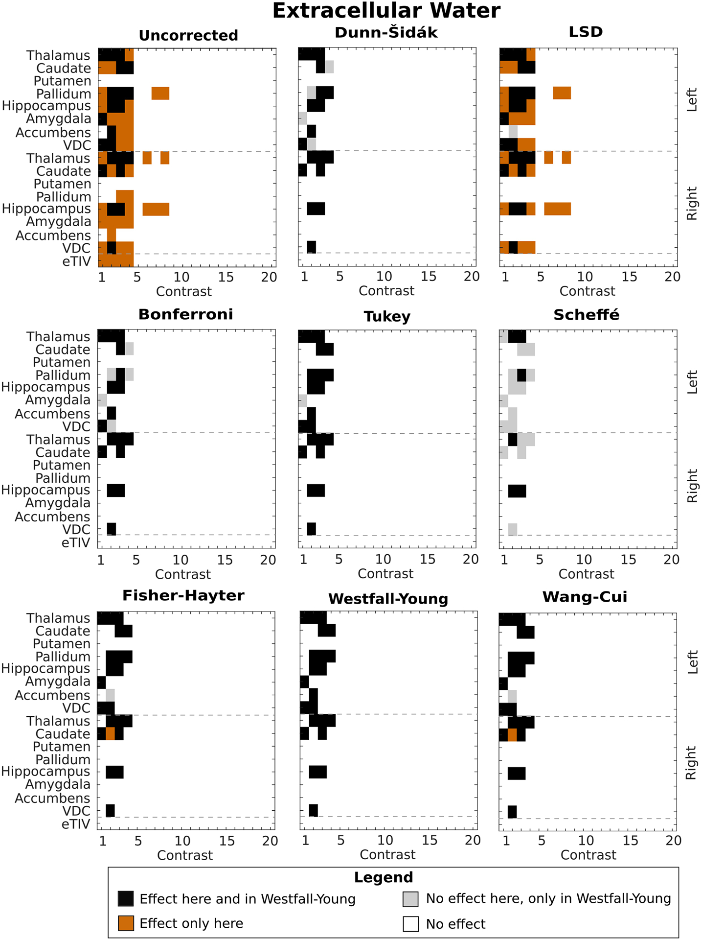
The multiple testing problem arises not only when there are many voxels or vertices in an image representation of the brain, but also when multiple contrasts of parameter estimates (that represent hypotheses) are tested in the same general linear model. We argue that a correction for this multiplicity must be performed to avoid excess of false positives. Various methods for correction have been proposed in the literature, but few have been applied to brain imaging. Here we discuss and compare different methods to make such correction in different scenarios, showing that one classical and well known method is invalid, and argue that permutation is the best option to perform such correction due to its exactness and flexibility to handle a variety of common imaging situations.

Keywords: Brain imaging; Contrast correction; Multiple comparisons; Multiple testing; Permutation tests.


Figures

Fig. A.1.
Fig. A.1.
Comparison between the correction performed with Bonferroni and Dunn–Šidák, where RB/DS = αBDS. Note that the ratio increases with the number of tests and decreases with the uncorrected level αunc used.
Fig. B.1.
Fig. B.1.
Signal distribution and its relation with the null distribution. Two signals with different powers are exhibited, one with 50% (a) and the other with 80% (b) power.
Fig. 1.
Fig. 1.
List of contrasts used to compare groups. Set 1 used C1 through C4, that is, testing whether G1 would have smaller gray matter volume than each one of the other four groups, whereas set 2 used C1 through C20, that is, testing all possible pairwise comparisons among the five groups (G1, …, G5) as encoded by the design matrix (not shown). The last two regression coefficients modelled age and sex, in an ancova design.
Fig. 2.
Fig. 2.
Mean familywise error rate and power after correcting across contrasts using Dunn–Šidák, Fisher lsd, Bonferroni, Tukey, Scheffé, Fisher–Hayter, West-fall-Young permutation method and Wang–Cui when testing all pairwise comparisons. Vertical bars represent the 95% confidence interval (tables with fwer and power, along with respective confidence intervals, are available in the Supplementary Material). Starting with balanced models, (a) shows the fwer results in the absence of signal when all contrasts are considered, (b) shows the fwer in the presence of signal, but considering the contrasts that have no signal, and (c) the respective power, i.e., the ability to detect signal for the contrasts that had signal; panels (d), (e), and (f) show, respectively, the same, for unbalanced models. A power of 50% was expected before any correction was performed.
Fig. 3.
Fig. 3.
Mean familywise error rate and power after correcting across contrasts using Dunn–Šidák, Fisher lsd, Bonferroni, Tukey, Scheffé, Fisher–Hayter, West-fall-Young permutation method and Wang–Cui when testing only a subset of linearly independent contrasts. Vertical bars represent the 95% confidence interval (tables with fwer and power, along with the respective confidence intervals, are available in the Supplementary Material). Starting with balanced models, (a) shows the fwer results in the absence of signal when all contrasts are considered, (b) shows the fwer in the presence of signal, but considering the contrasts that have no signal, and (c) the respective power, i.e., the ability to detect signal for the contrasts that had signal; panels (d), (e), and (f) show, respectively, the same, for unbalanced models. A power of 20.6% was expected before any correction was performed.
Fig. 4.
Fig. 4.
Effects in both hemispheres per contrast detected when dividing the subjects into five groups using the percentiles from bsmss and testing contrast set 1, that is, when testing whether subjects with lower scores of bsmss (group 1) have smaller cortical volume than subjects from the other four groups (with higher scores of BSMSS). Contrast 1 tests if group 1 has smaller volume than group 2, contrast 2 tests if group 1 has smaller volume than group 3, and so forth (see Fig. 1 for the list of contrasts tested).
Fig. 5.
Fig. 5.
Effects in both hemispheres per contrast detected when dividing the subjects into five groups using the percentiles from bsmss and all 20 pairwise comparisons were considered (contrast set 2). Before the correction across contrasts, some effects were detected (left panel), but no effect survived the correction performed with any of evaluated methods.
Fig. 6.
Fig. 6.
Effects in both hemispheres per contrast detected when dividing the subjects into five groups using the percentiles from extracellular water and testing contrast set 1, that is, testing whether subjects with lower extracellular water volume (group 1) have smaller cortical volume than subjects from the other 4 groups (with higher scores of extracellular water volume). Contrast 1 tests if group 1 has smaller volume than group 2, contrast 2 tests if group 1 has smaller volume than group 3, and so forth (see Fig. 1 for the list of contrasts tested).
Fig. 7.
Fig. 7.
Effects in both hemispheres per contrast detected when dividing the subjects into five groups using the percentiles from extracellular water and all 20 pairwise comparisons were considered (contrast set 2).

Similar articles

Cited by

References

    1. Abdi H, 2007. The bonferonni and Šidák corrections for multiple comparisons. In: Encyclopedia of Measurement and Statistics. SAGE, pp. 1–9.
    1. Alexander LM, Escalera J, Ai L, Andreotti C, Febre K, Mangone A, Vega-Potler N, Langer N, et al., 2017. Data Descriptor: an open resource for transdiagnostic research in pediatric mental health and learning disorders. Scientific Data 4, 1–26. - PMC - PubMed
    1. Barch DM, Burgess GC, Harms MP, Petersen SE, Schlaggar BL, Corbetta M, Glasser MF, Curtiss S, Dixit S, Feldt C, et al., 2013. Function in the human connectome: task-fmri and individual differences in behavior. Neuroimage 80, 169–189. - PMC - PubMed
    1. Barratt W, 2006. The Barratt Simplified Measure of Social Status (BSMSS): Measuring SES. Indiana State University, Unpublished manuscript.
    1. Bonferroni C, 1936. Teoria statistica delle classi e calcolo delle probabilita. Pubblicazioni del R Istituto Superiore di Scienze Economiche e Commericiali di Firenze 8, 3–62.

Publication types