Generalization error analysis for deep convolutional neural network with transfer learning in breast cancer diagnosis

Abstract

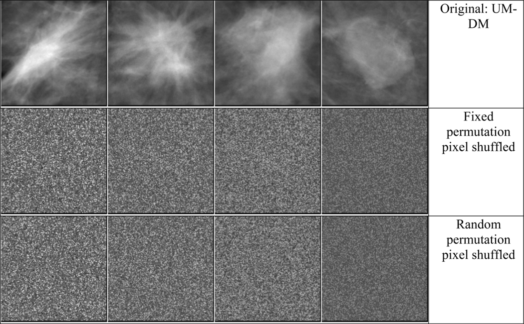
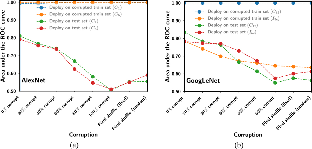
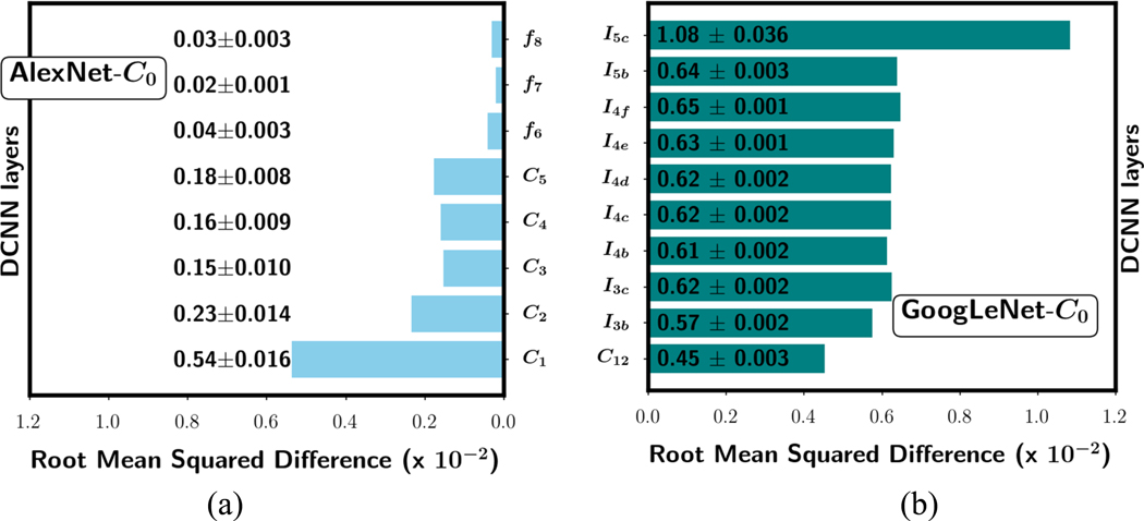
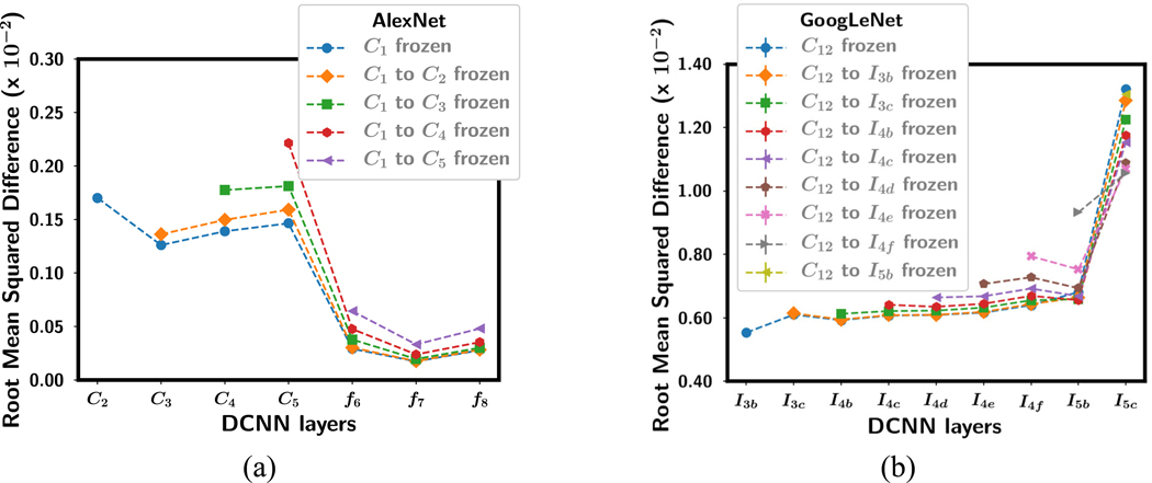
Deep convolutional neural network (DCNN), now popularly called artificial intelligence (AI), has shown the potential to improve over previous computer-assisted tools in medical imaging developed in the past decades. A DCNN has millions of free parameters that need to be trained, but the training sample set is limited in size for most medical imaging tasks so that transfer learning is typically used. Automatic data mining may be an efficient way to enlarge the collected data set but the data can be noisy such as incorrect labels or even a wrong type of image. In this work we studied the generalization error of DCNN with transfer learning in medical imaging for the task of classifying malignant and benign masses on mammograms. With a finite available data set, we simulated a training set containing corrupted data or noisy labels. The balance between learning and memorization of the DCNN was manipulated by varying the proportion of corrupted data in the training set. The generalization error of DCNN was analyzed by the area under the receiver operating characteristic curve for the training and test sets and the weight changes after transfer learning. The study demonstrates that the transfer learning strategy of DCNN for such tasks needs to be designed properly, taking into consideration the constraints of the available training set having limited size and quality for the classification task at hand, to minimize memorization and improve generalizability.

Fig. 1.

DCNN structures of AlexNet (top) and GoogLeNet (bottom). The input is an image patch of size 256 × 256 pixels and the output is a binary classification of 0 (benign) and 1 (malignant).

Fig. 2.

Examples of mass ROIs of from SFM and DM and the corresponding pixel shuffled ROIs. Left two masses are malignant and right two masses are benign.

Fig. 2.

Examples of mass ROIs of from SFM and DM and the corresponding pixel shuffled ROIs. Left two masses are malignant and right two masses are benign.

Fig. 3.

Four-fold cross-validation results of transfer learning networks for AlexNet and GoogLeNet. All experiments were repeated five times to assess the sensitivity of the DCNN to random stochastic initialization of the weights. The test AUCs for the four folds were plotted offset horizontally to facilitate viewing. The mean across the folds is indicated by the blue dotted line. The horizontal axis label represents the layer (or inception block) up to which the layers were frozen during transfer learning: C₀ indicates all the layers were allowed to train, C_n (or F_n, I_n) indicates layers up to C_n (or F_n , I_n) were frozen and the rest of the layers were allowed to train. The input training data was uncorrupted. The best test AUC was observed when the first convolutional layer was frozen achieving average AUCs of 0.81±0.04 and 0.83±0.03 for AlexNet and GoogLeNet, respectively, in the four-fold cross-validation.

Fig. 4.

Learning curves for classifying breast masses with label corruption by AlexNet (top row) and GoogLeNet (bottom row). (a) and (c) are for transfer network with only the first convolutional layer frozen. (b) and (d) are for transfer network with all convolutional layers frozen. Each data point shows the mean and the standard deviation estimated from the four training AUCs from the 4-fold cross-validation. Note the difference in the range of the horizontal axis between the top and bottom rows.

Fig. 5.

Learning curves for classifying breast mass images corrupted by pixel shuffling (fixed and random permutation) by (a) AlexNet and (b) GoogLeNet using two transfer learning networks each. Each data point shows the mean and the standard deviation estimated from the four training AUCs from the 4-fold cross-validation. Note the difference in the range of the horizontal axis between (a) and (b). The AlexNet-C₅ curves eventually reached a training AUC of 1 at over 1000 epochs.

Fig. 6.

Generalization error between training and test obtained as the mean AUC of the training sets and the corresponding mean AUC of the test sets from 4-fold cross-validation for the various amount or type of corruption on the training set. The test sets were not corrupted. (a) AlexNet, (b) GoogLeNet for two transfer learning networks each.

Fig. 7.

Mean RMSD of the weight changes in each layer averaged over the four training folds for (a) AlexNet-C₀ and (b) GoogLeNet-C₀ networks after transfer learning. The mean and standard deviation values for each layer are shown for the corresponding bar. The training set was uncorrupted and none of the layers was frozen during transfer learning.

Fig. 8.

Mean RMSD of the weight changes in each layer averaged over the four training folds for (a) AlexNet and (b) GoogLeNet after transfer learning with uncorrupted data. The standard deviations were in the range of 0.001 to 0.03, smaller than the symbols of the data points, so that they were not plotted. The convolutional layers that were frozen during training were shown in the legend. Note that the horizontal axis shows the DCNN layer where the RMSD shown in the vertical axis was calculated. The RMSD value of the frozen layers was zero and not plotted. Note the difference in the scaling of the vertical axis between (a) and (b).

Fig. 9.

Mean RMSD of the weight changes in each layer averaged over the four training folds for (a) AlexNet-C₁ and (b) GoogLeNet-C₁₂ with the first convolutional layer frozen after transfer learning with corrupted data. The standard deviations were in the range of 0.001 to 0.03, smaller than the symbols of the data points, so that they were not plotted. The horizontal axis shows the DCNN layer where the RMSD shown in the vertical axis was calculated. Note the difference in the scaling of the vertical axis between (a) and (b).

References

1. Antropova N, Huynh B Q and Giger M L 2017. A deep feature fusion methodology for breast cancer diagnosis demonstrated on three imaging modality datasets Medical physics 44 5162–71 - PMC - PubMed
1. Byra M, Styczynski G, Szmigielski C, Kalinowski P, Michałowski Ł, Paluszkiewicz R, Ziarkiewicz-Wróblewska B, Zieniewicz K, Sobieraj P and Nowicki A 2018. Transfer learning with deep convolutional neural network for liver steatosis assessment in ultrasound images Int J Comput Ass Rad 13 1895–903 - PMC - PubMed
1. Chan H-P, Lo S C, Helvie M, Goodsitt M M, Cheng S N C and Adler D D 1993. Recognition of mammographic microcalcifications with artificial neural network Radiology 189(P) 318
1. Chan H-P, Lo S C B, Sahiner B, Lam K L and Helvie M A 1995a. Computer-aided detection of mammographic microcalcifications: Pattern recognition with an artificial neural network Medical Physics 22 1555–67 - PubMed
1. Chan H-P, Sahiner B, Lo S C, Helvie M, Petrick N, Adler D D and Goodsitt M M 1994. Computer-aided diagnosis in mammography: detection of masses by artificial neural network Medical Physics 21 875–6
Publication types