. 2020 Mar;579(7800):567-574.
doi: 10.1038/s41586-020-2095-1. Epub 2020 Mar 11.

Microbiome analyses of blood and tissues suggest cancer diagnostic approach

Affiliations

Microbiome analyses of blood and tissues suggest cancer diagnostic approach

Gregory D Poore et al. Nature. 2020 Mar.

Retraction in

Abstract

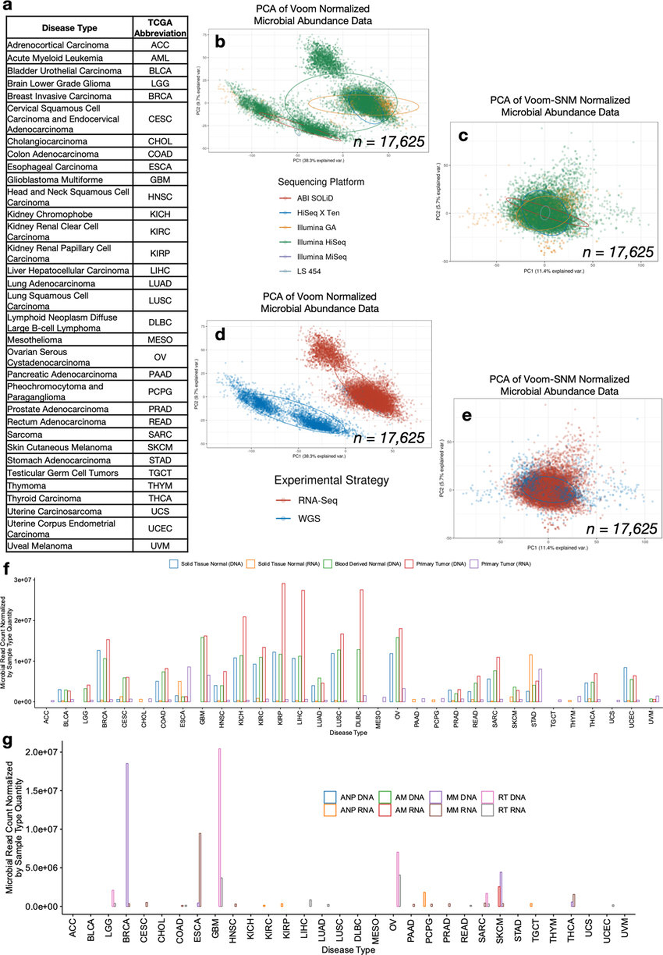
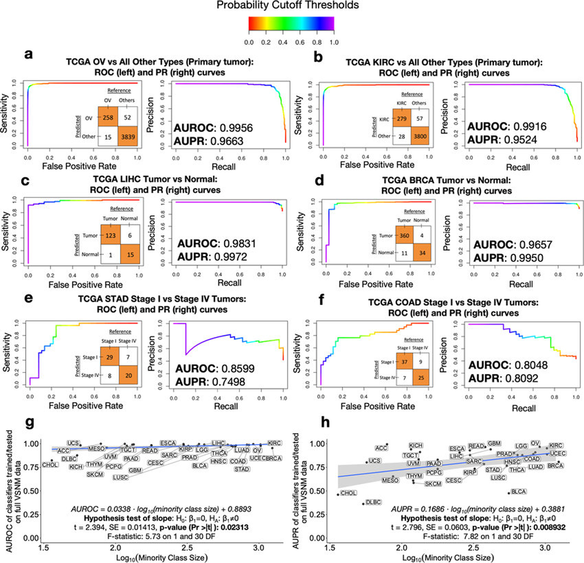
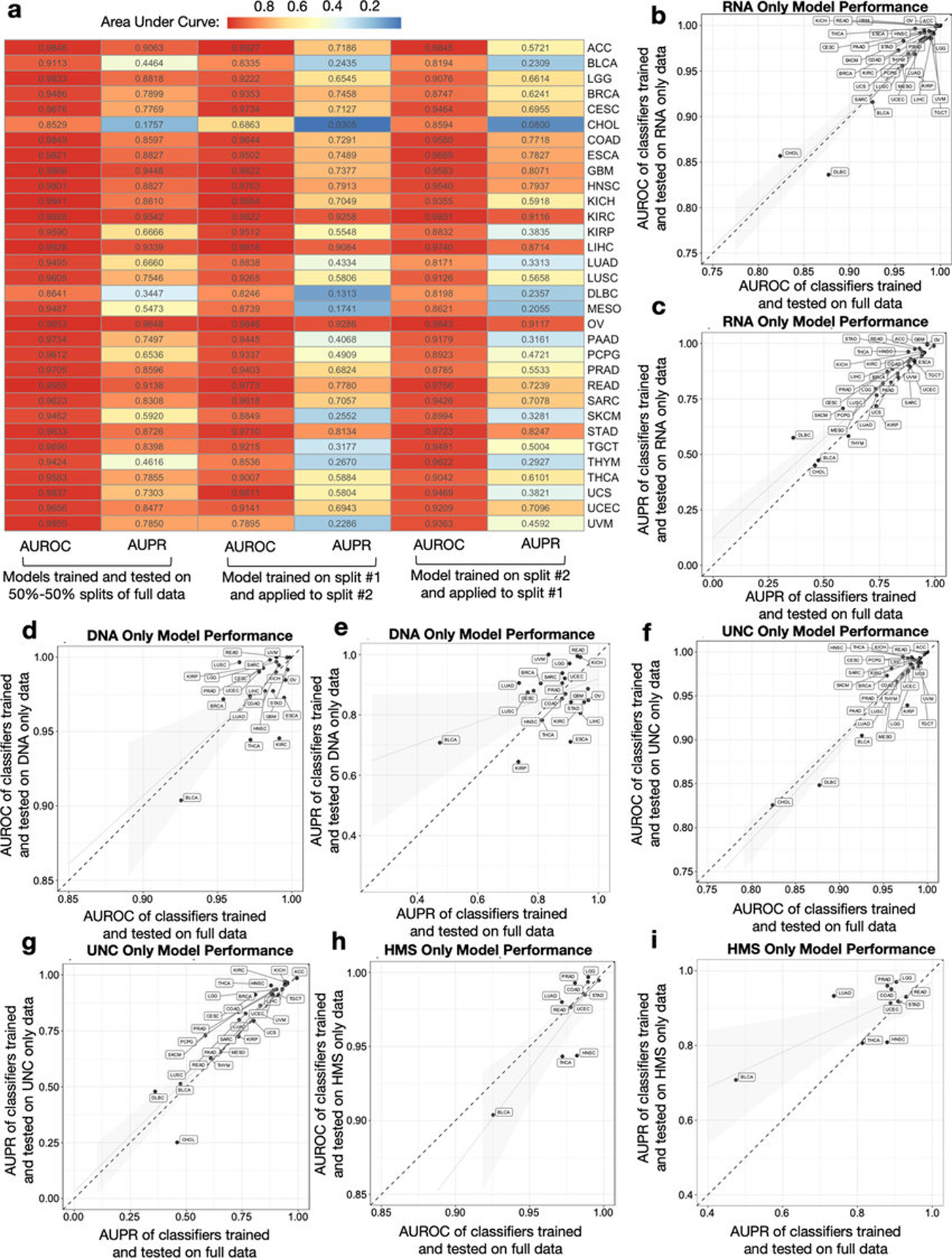
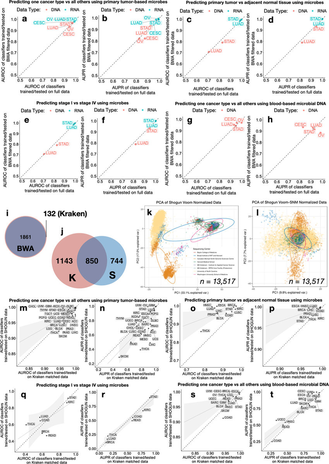
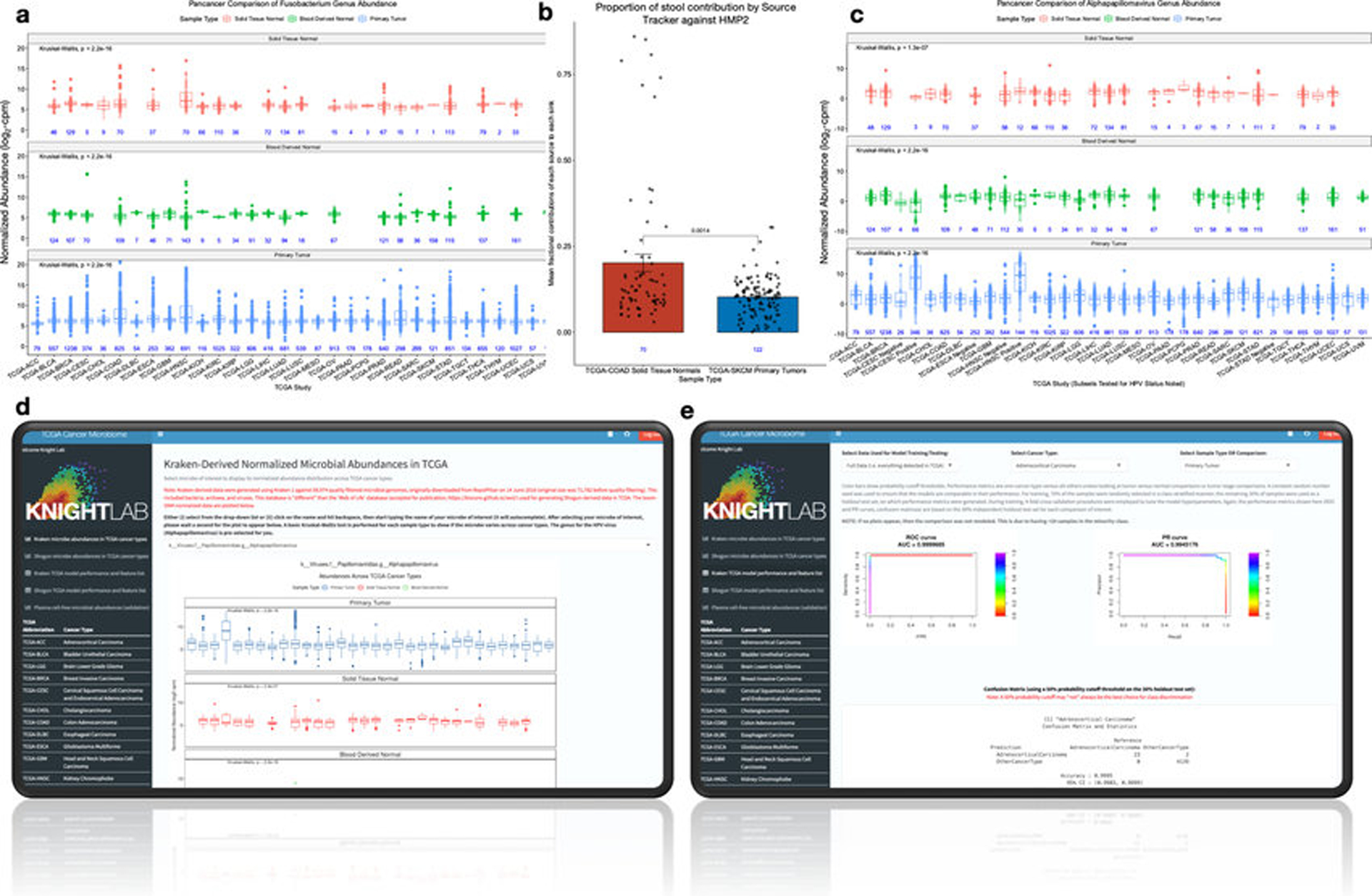
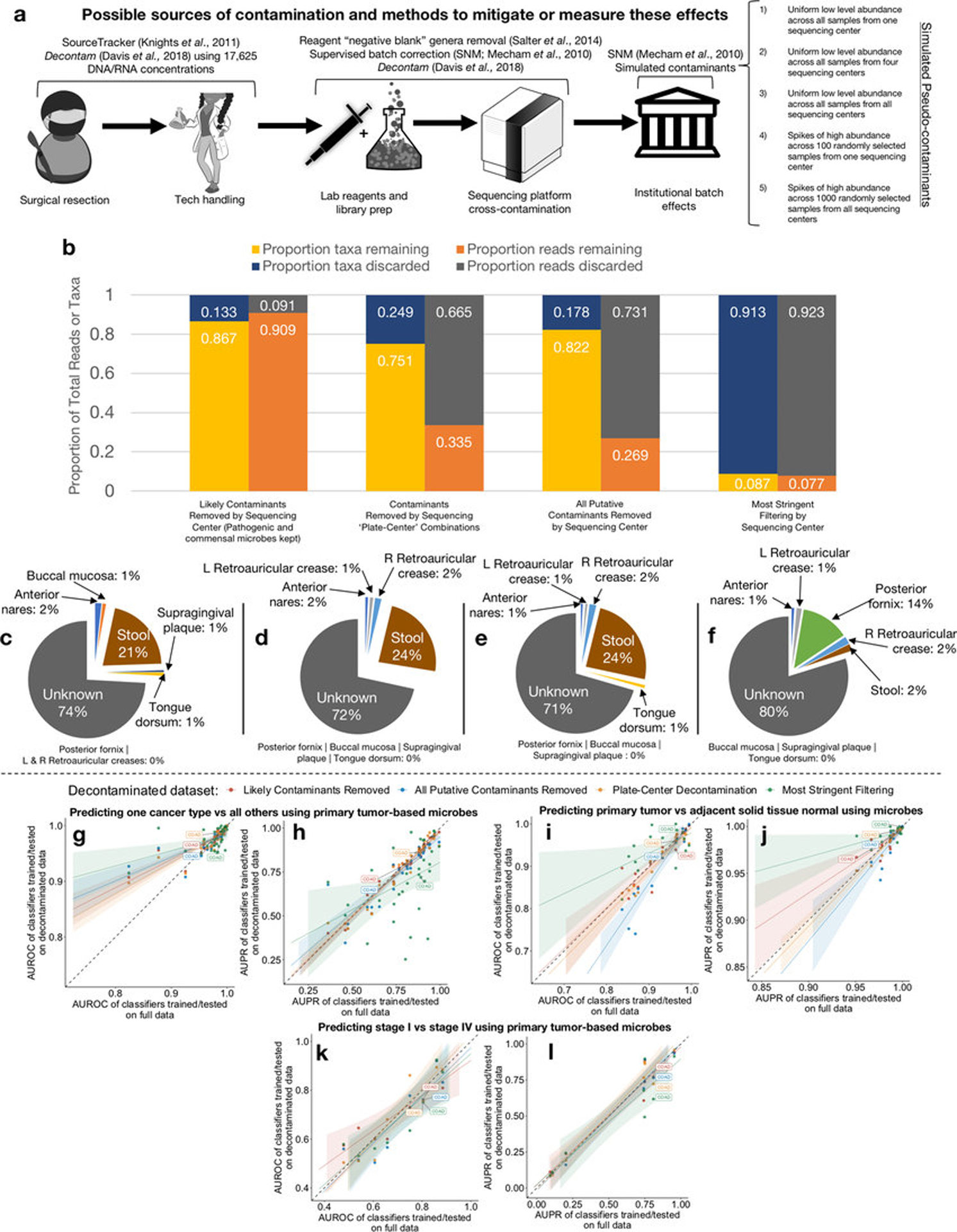
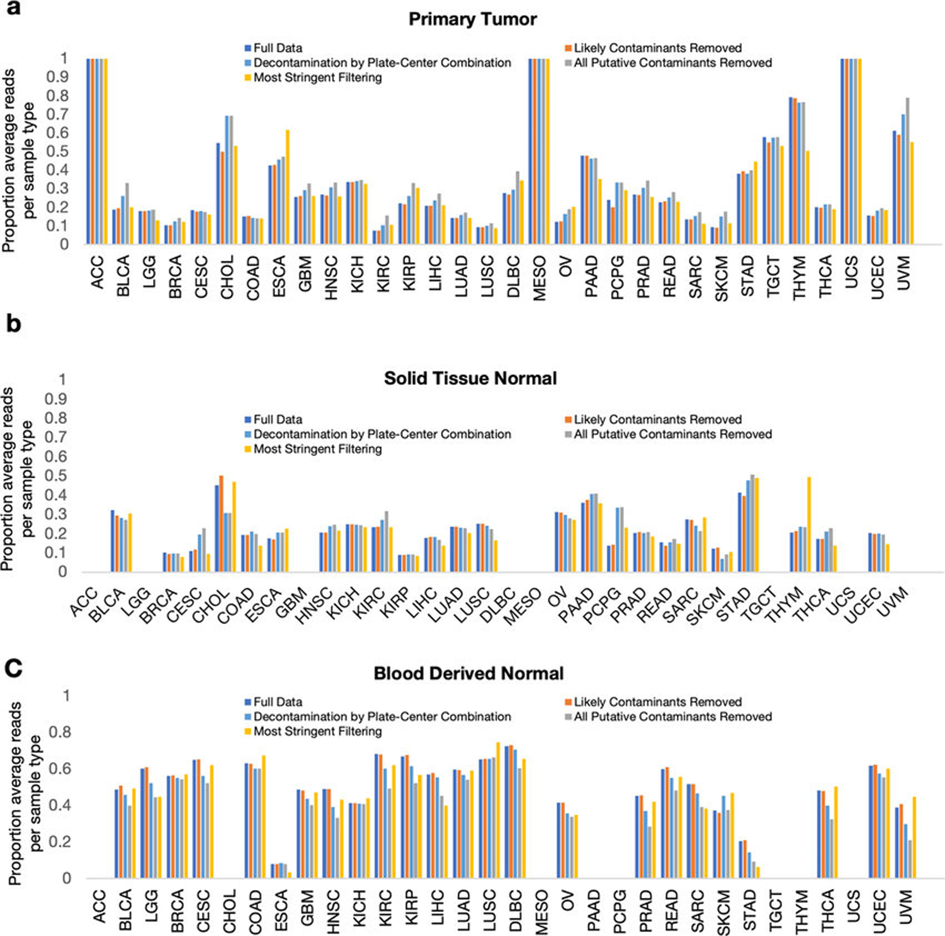
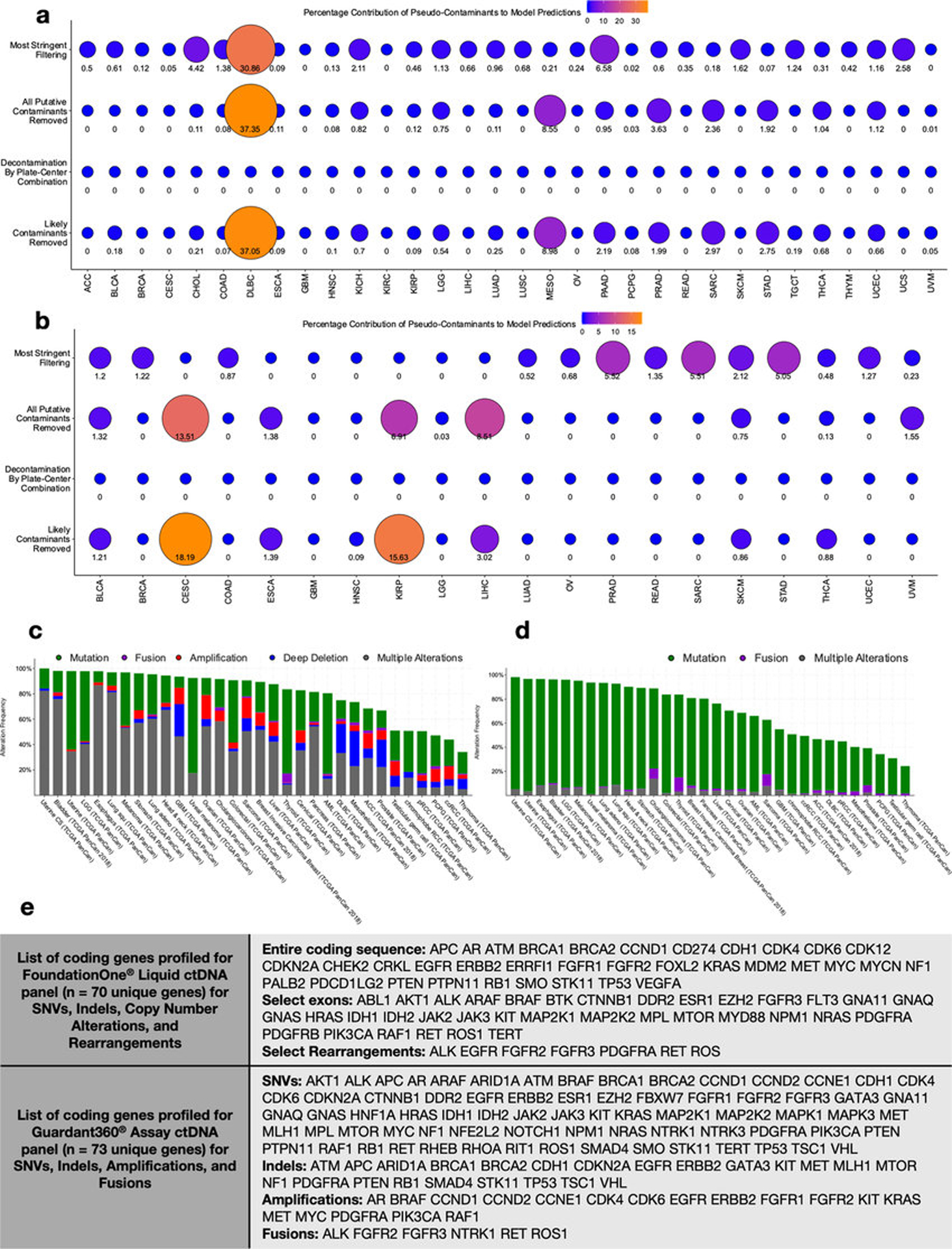
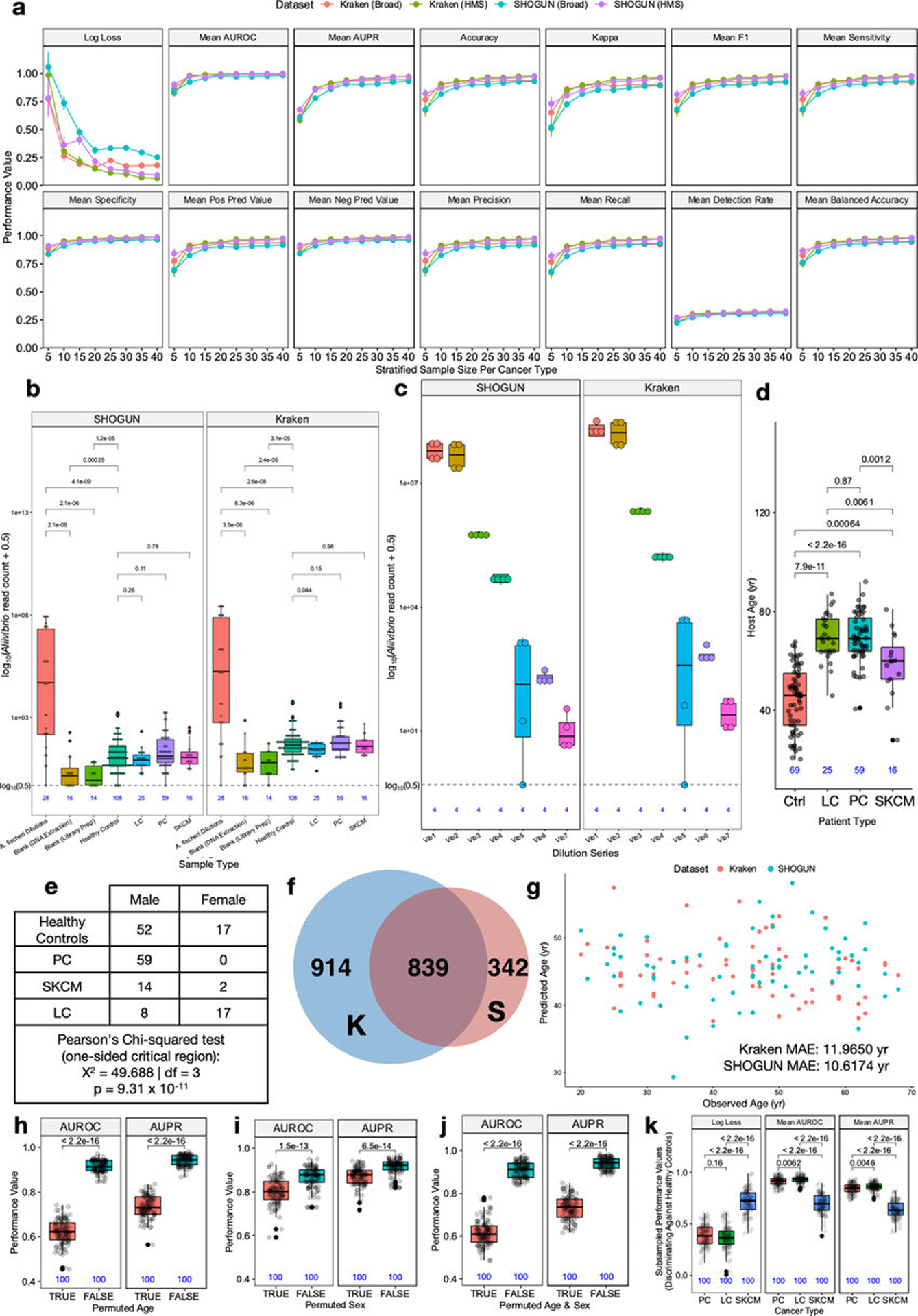
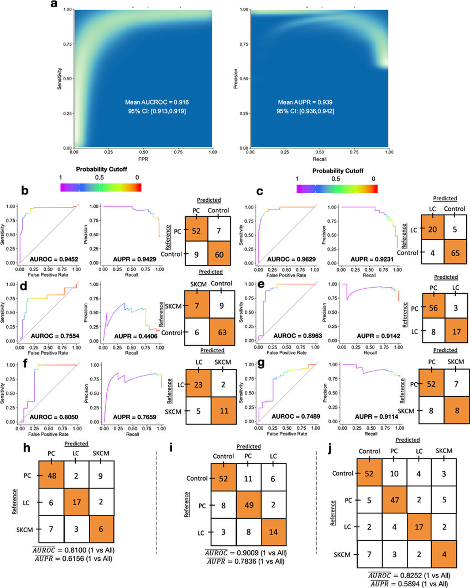
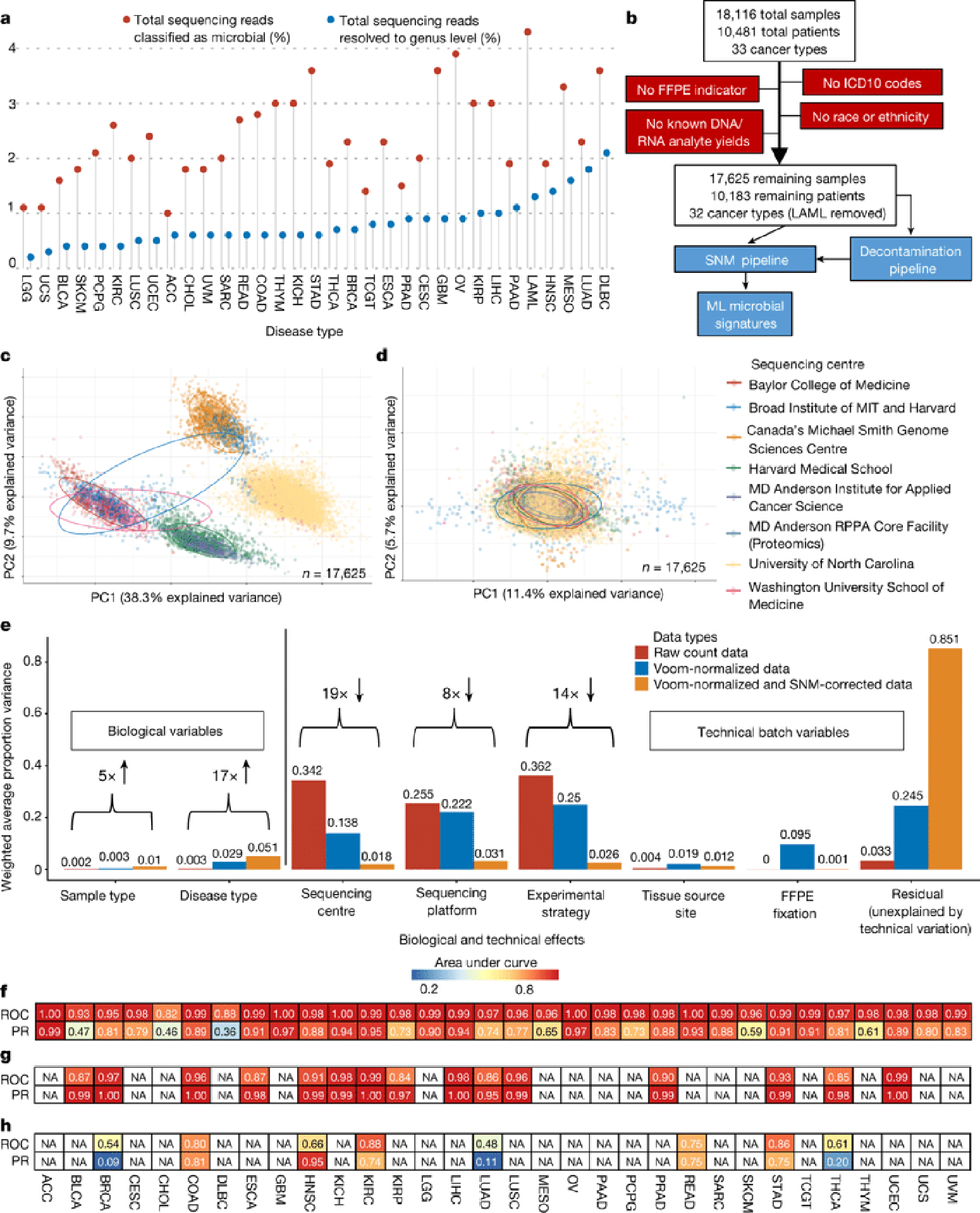
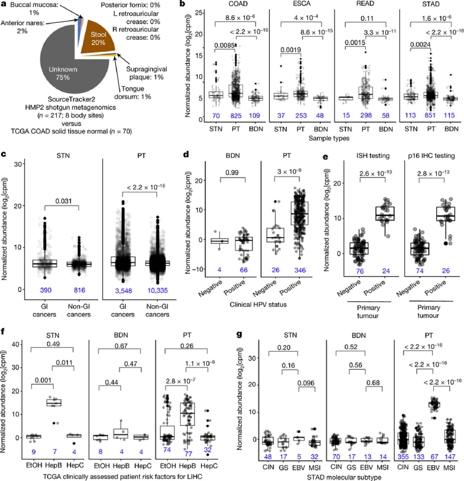
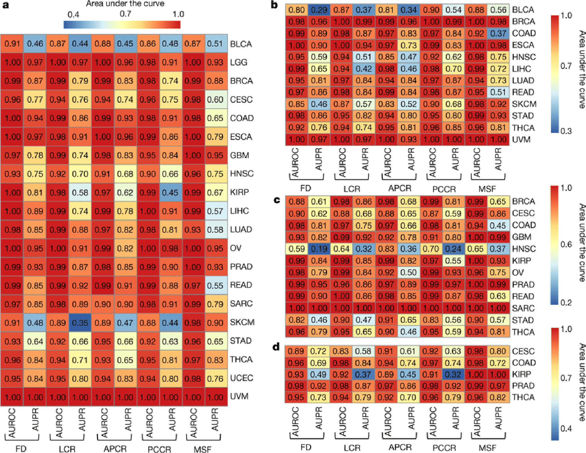
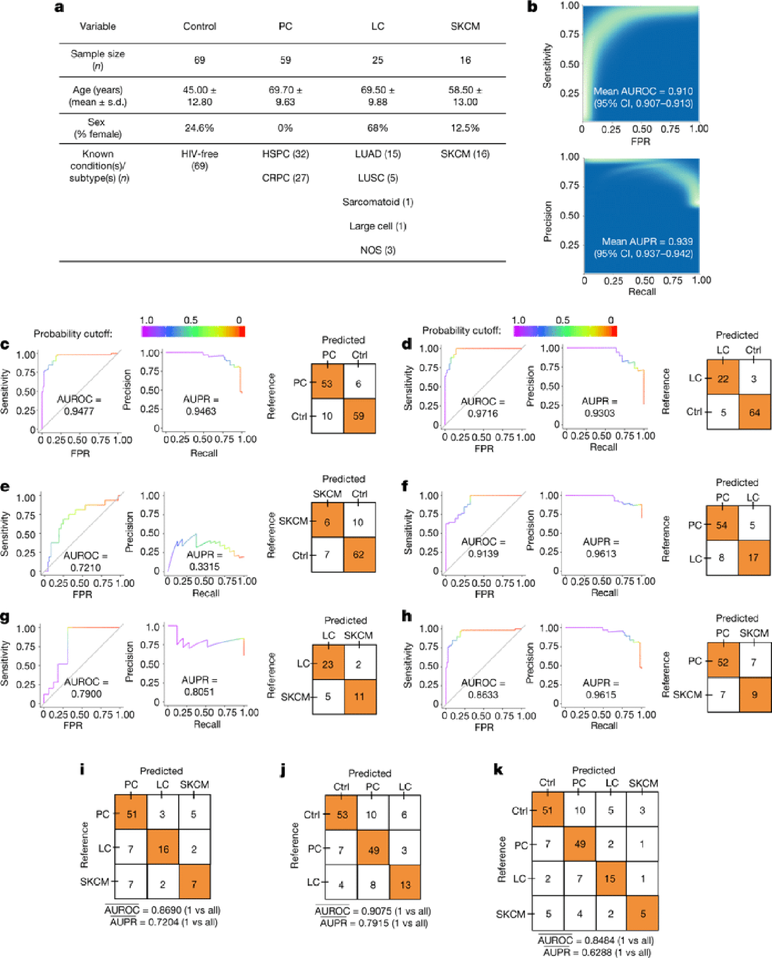
Systematic characterization of the cancer microbiome provides the opportunity to develop techniques that exploit non-human, microorganism-derived molecules in the diagnosis of a major human disease. Following recent demonstrations that some types of cancer show substantial microbial contributions1-10, we re-examined whole-genome and whole-transcriptome sequencing studies in The Cancer Genome Atlas11 (TCGA) of 33 types of cancer from treatment-naive patients (a total of 18,116 samples) for microbial reads, and found unique microbial signatures in tissue and blood within and between most major types of cancer. These TCGA blood signatures remained predictive when applied to patients with stage Ia-IIc cancer and cancers lacking any genomic alterations currently measured on two commercial-grade cell-free tumour DNA platforms, despite the use of very stringent decontamination analyses that discarded up to 92.3% of total sequence data. In addition, we could discriminate among samples from healthy, cancer-free individuals (n = 69) and those from patients with multiple types of cancer (prostate, lung, and melanoma; 100 samples in total) solely using plasma-derived, cell-free microbial nucleic acids. This potential microbiome-based oncology diagnostic tool warrants further exploration.


Conflict of interest statement

Competing interests

Clarity Genomics, the employer of E.K., did not provide funding for this study. Both G.D.P. and R.K. have jointly filed U.S. Provisional Patent Application Serial No. 62/754,696 and International Application No. PCT/US19/59647 on the basis of this work. G.D.P., R.K., and S.M.M. have started a company to commercialize the intellectual property. R.K. is a member of the SAB for GenCirq, Inc., holds an equity interest in GenCirq, and can receive reimbursements for expenses up to $5,000/yr. R.K., A.D.S., and S.M.M. are directors at the Center for Microbiome Innovation at UC San Diego, which receives industry research funding for various microbiome initiatives, but no industry funding was provided for this cancer microbiome project.

Figures

Extended Data Figure 1:
Extended Data Figure 1:. Continued overview of the TCGA cancer microbiome.
a, TCGA study abbreviations. b, Principal components analysis (PCA) of Voom normalized data, where colors represent sequencing platform of the sample and each dot denotes a cancer microbiome sample. c, PCA of the data following consecutive Voom-SNM supervised normalization, as labeled by sequencing platform. d, PCA of Voom normalized data, where colors represent experimental strategy of the sample and each dot denotes a cancer microbiome sample. e, PCA of the data following consecutive Voom-SNM supervised normalization, as labeled by experimental strategy. f-g, Microbial reads counts as normalized by the quantity of samples within a given sample type across all cancer types in TCGA after metadata quality control (Fig. 1b), including the three major sample types analyzed in the paper (f) and the remaining sample types (g). Note the following abbreviations: ANP = Additional - New Primary; AM = Additional Metastatic; MM = Metastatic; RT = Recurrent Tumor.
Extended Data Figure 2:
Extended Data Figure 2:. Performance metrics details discriminating between and within TCGA cancer types using microbial abundances.
a-f, Expanded examples from the heatmaps in Figs. 1f–h. A color gradient shown at the top denotes the probability threshold at any point along the ROC and PR curves. An inset confusion matrix is shown using a 50% probability threshold cutoff, which can be used to calculate sensitivity, specificity, precision, recall, positive predictive value, negative predictive values, and so forth at the corresponding point on the ROC and PR curves. g-h, Linear regressions of model performance, specifically AUROC (g) and AUPR (h), for discriminating between cancer types in a one-cancer-type-versus-all-others manner, as a function of minority class size. Performances are shown for models using microbes detected in primary tumors, which had the greater number of samples (n=13,883) and cancer types (n=32) to compare. Since AUROC and AUPR have domains of [0,1] and the minority class size varied from 20 to 1238 samples, the latter is regressed on a log10 scale. Inset hypothesis tests and associated p-values are based on the null hypothesis of there being no relationship between the dependent and independent variables (two-sided test).
Extended Data Figure 3:
Extended Data Figure 3:. Internal validation of ML model pipeline.
a, Two independent halves of TCGA raw microbial count data were normalized and used for model training to predict one-cancer-type-versus-all-others using tumor microbial DNA and RNA; each model was then applied on the other half’s normalized data. This heatmap compares the performances of these models as compared to training and testing on 50%−50% splits of the full dataset. b-c, Model performance comparison when subsetting the full Voom-SNM data by primary tumor RNA samples (n=11,741) across multiple sequencing centers to predict one-cancer-type-versus-all-others. d-e, Model performance comparison when subsetting the full Voom-SNM data by primary tumor DNA samples (n=2142) across multiple sequencing centers to predict one-cancer-type-versus-all-others. f-g, Model performance comparison when subsetting the full Voom-SNM data by University of North Carolina (UNC) samples (n=9726), which only did RNA-Seq, to predict one-cancer-type-versus-all-others using primary tumor RNA samples. h-i, Model performance comparison when subsetting the full Voom-SNM data by from Harvard Medical School (HMS) samples (n=898), which only did WGS, to predict one-cancer-type-versus-all-others using primary tumor DNA samples. For all models in b-i: Generalized linear models with standard errors are shown in gray; the dotted diagonal line denotes a perfect linear relationship; for sample size comparison, the full Voom-SNM dataset contained 13,883 primary tumor samples.
Extended Data Figure 4:
Extended Data Figure 4:. Orthogonal validation of Kraken-derived TCGA cancer microbiome profiles and their ML performances.
a-h, Four TCGA cancer types (CESC, STAD, LUAD, OV) underwent additional filtering after Kraken-based taxonomy assignments via direct genome alignments (Burrows-Wheeler Aligner, BWA). ML performances are compared between the normalized, BWA filtered data and matched, independently normalized Kraken data for one-cancer-type-versus-all-others using primary tumor microbes (a-b), tumor-versus-normal discriminations (c-d), stage I versus stage IV tumor discriminations using primary tumor microbes (e-f), and one-cancer-type-versus-all-others using blood-derived microbes (g-h) (Methods). i, Venn diagram of the taxa count between the BWA filtered data and the Kraken “full” data. j-t, An orthogonal microbial-detection pipeline called SHOGUN (“SHallow shOtGUN sequencing”) that uses direct genome alignments and a separate database (‘Web of Life’ [WoL]; n=10,575 microbial genomes [bacteria, archaea]; https://biocore.github.io/wol/) was run on a subset of TCGA samples covering every analyzed cancer type (n=32), sample type (n=7), sequencing platform (n=6), and sequencing center (n=8) in the Kraken-based analysis (n=13,517 total samples). SHOGUN-derived microbial count data were normalized via Voom-SNM, analogous to its Kraken counterpart, and utilized for downstream ML analyses. j, Venn diagram of the SHOGUN-derived microbial taxa and the Kraken-derived microbial taxa. Note the use of separate databases and the fact that WoL does not include viruses while the Kraken database does. k-l, PCA of Voom (k) and Voom-SNM (l) normalized SHOGUN data, colored by sequencing center. m-t, ML performance comparisons between models trained and tested on SHOGUN data and matched Kraken data, using the same 70%/30% splits, for one-cancer-type-versus-all-others using primary tumor microbes (m-n), tumor-versus-normal discriminations (o-p), stage I versus stage IV tumor discriminations using primary tumor microbes (q-r), and one-cancer-type-versus-all-others using blood-derived microbes (s-t). For fair comparison, matched Kraken data were derived by removing all virus assignments in the raw Kraken count data and subsetting to the same 13,517 TCGA samples analyzed by SHOGUN; these matched Kraken data were then normalized independently via Voom-SNM the exact same way as the SHOGUN data (Methods) and fed into downstream ML pipelines. For all ML performances: A minimum minority class sample size of 20 was required to be eligible. For regression subfigures: The dotted diagonal line denotes perfect performance correspondence; generalized linear models with standard error ribbons are shown.
Extended Data Figure 5:
Extended Data Figure 5:. Pan-cancer microbial abundances and an interactive website for TCGA cancer microbiome profiling and ML model inspection.
a, Pan-cancer Fusobacterium normalized abundances with a one-way ANOVA (Kruskal-Wallis) test for microbial abundances across cancer types for each sample type. Sample sizes are inset in blue, and TCGA study names are listed at the bottom. b, SourceTracker2 results for fecal contribution, as based on HMP2 data, for TCGA-COAD solid-tissue normal samples and TCGA-SKCM primary tumor samples. Only 1 solid tissue normal sample was available for TCGA-SKCM (Table S4), so primary tumors were used instead as the best proxy of expected skin flora. It is expected that colon samples should have higher fecal contribution than skin, so a one-sided Mann-Whitney test was employed. Since SourceTracker2 outputs mean fractional contributions of each source (i.e. HMP2) to each sink (i.e. COAD, SKCM samples), the center value of each bar plot is the mean of these values and the error bars denote the standard error. The sample sizes are inset below the bars in blue. c, Pan-cancer Alphapapillomavirus normalized abundances with a one-way ANOVA (Kruskal-Wallis) test for microbial abundances across cancer types for each sample type. Sample sizes are inset in blue, and TCGA study names are listed at the bottom. TCGA studies that clinically tested patients for HPV infection have “negative” or “positive” appended depending on the result of the test. d, Interactive website screenshot showing plotting of Alphapapillomavirus normalized microbial abundances using Kraken-derived data. Plotting using SHOGUN-derived normalized microbial abundances is available on another tab of the website (left-hand side). e, Interactive website screenshot of ML model inspection. Selecting the data type (e.g. all likely contaminants removed), cancer type (e.g. invasive breast carcinoma), and comparison of interest (e.g. tumor vs normal) will automatically update the ROC and PR curves, as well as the confusion matrix (using a probability cutoff threshold of 50%) and the ranked model feature list. Website is accessible at http://cancermicrobiome.ucsd.edu/CancerMicrobiome_DataBrowser/. All box plots show median, 25th and 75th percentiles, and whiskers that extend to 1.5× the interquartile range.
Extended Data Figure 6:
Extended Data Figure 6:. The decontamination approach along with its results, benefits, and limitations on cancer microbiome data.
a, Various approaches used to either evaluate, mitigate, remove and/or simulate sources of contamination. b, The proportion of remaining taxa or microbial reads in TCGA after varying levels of decontamination. Decontamination by “sequencing center” removed all taxa identified as a contaminant at any one sequencing center (n=8 ‘batches’); decontamination by “plate-center” combinations removed all taxa identified as a contaminant on any one single sequencing plate having more than 10 TCGA samples on it (n=351 ‘batches’). c-f, Body-site attribution prediction on the “likely contaminants removed” dataset (c), the “plate-center decontaminated” dataset (d), the “all putative contaminants removed” dataset (e), and the “most stringent filtering” dataset (f). g-l, All of the models and concomitant performance values (AUROC and AUPR) were re-generated using the four decontaminated datasets described above (each labeled with a different color; see legend located above plots). The AUROC and AUPR values obtained from models trained and tested on the decontaminated datasets are plotted against the AUROC or AUPR values from the “full” dataset (shown in Figs. 1f–h). The dashed diagonal line denotes a perfect linear relationship. Generalized linear models have been fitted to the corresponding datasets’ AUROC and AUPR values; standard errors of the linear fits are shown by the associated shaded regions. COAD model performances are identified throughout the figures.
Extended data figure 7:
Extended data figure 7:. Decontamination effects on proportion of average reads per sample type.
a-c, The total read count (i.e. DNA and RNA) of each major sample type (primary tumor [a], solid-tissue normal [b], blood-derived normal [c]) was summed and divided by the total number of samples within each sample type. This normalized read count (per sample type) was then divided by the summed normalized read count across all sample types for each cancer type, thereby providing an estimate of the proportion of average reads per sample type per cancer type. This was repeated for all five datasets, as shown by the legend, to assess if decontamination differentially impacts certain sample types and/or certain cancer types; relative stability in the percentages shown would suggest a lack of differential contamination. Minor sample types that were not further analyzed in this paper by decontamination or ML (e.g. additional metastatic lesions; n=4 sample types; Extended Data Fig. 1g) are not shown and comprised only 3.80% of total TCGA samples. Note, in the special case that only one sample type exists for a given cancer type (i.e. primary tumor in ACC, MESO, UCS), then all bars will show that 100% of the normalized reads came from that one sample type.
Extended data figure 8:
Extended data figure 8:. Measuring spiked pseudo-contaminant contribution in downstream ML models and theoretical sensitivities of commercially available, host-based, cell-free DNA (ctDNA) assays in TCGA patients.
a-b, Feature importance scores were calculated for all taxa used in models trained to discriminate one-cancer-type-versus-all-others in all four decontaminated datasets (Extended Data Fig. 6b) using primary tumor microbial DNA or RNA (a), or using blood-derived mbDNA (b). These decontaminated datasets were spiked with pseudo-contaminants prior to the decontamination and normalization pipelines to evaluate their performance (Methods), and the test set performances of the models shown are given in Extended Data Figs. 6g–h and Fig. 3a, respectively. Any spiked pseudo-contaminant(s) used by a model had their feature importance score(s) divided by the sum total of all feature importance scores in that model to estimate a percentage contribution of them towards making accurate predictions; the higher the score (out of 100), the less biologically reliable the model is. Note, “0” means that no spiked pseudo-contaminants were used for making predictions by the model; none of the models generated on the “plate-center decontaminated” data included spiked pseudo-contaminants as features. c-d, Percent distribution among TCGA studies with patients having one or more genomic alterations on FoundationOne® Liquid ctDNA coding genes (c) or on Guardant360® ctDNA coding genes (d). Data are downloaded from https://www.cbioportal.org/. e, The specific list of coding genes for the FoundationOne® and Guardant360® ctDNA assays and their examined alterations (source listed in Methods).
Extended Data Figure 9:
Extended Data Figure 9:. Supporting analysis for real-world, plasma-derived, cell-free microbial DNA analysis between and among healthy individuals and multiple cancer types.
a, Discriminatory simulations in TCGA used to empirically power the real-world validation study (Fig. 4; Methods for details) and the theoretical performance metrics for each stratified sample size (per cancer type) using blood samples from the three cancer types of interest (prostate cancer (PC), lung cancer (LC), melanoma (SKCM)). Center values for each stratified sample size are the means of the performances and error bars denote the standard errors. Stratified sampling means that a sample size of five per cancer type would be a total of 15 blood samples under study for three-class discrimination (Methods). TCGA blood-derived normal samples were subsetted from The Broad Institute (Broad) and Harvard Medical School (HMS) such that they came from one sequencing center (i.e. Broad or HMS), one sequencing platform (Illumina HiSeq), and one experimental strategy (WGS). The two kinds of LC in TCGA (LUAD, LUSC) were combined to reflect the samples available for the validation study. The resultant Broad and HMS datasets, as raw microbial counts, were then normalized separately via Voom-SNM, as would be in the validation study, and fed into a multi-class (n=3), leave-one-out (LOO) ML pipeline. Ten permuted iterations per stratified sample size per cancer type were used to estimate standard errors of theoretical performance estimates; for example, a stratified sample size of 40 would involve training and testing 1200 ML models ( = 40 samples * 3 cancer types * 10 iterations), from which 10 performance estimates would be made on 120 samples each to estimate standard errors (see Methods for details). All of this was repeated for SHOGUN-derived data as well. b, Evaluation of Aliivibrio genus abundance values (raw read counts) among positive control bacterial (Aliivibrio) monocultures, negative control blanks, and human sample types using both Kraken and SHOGUN-derived taxonomy assignments. Note the log10 scale and 0.5 pseudo-count lower limit, shown with a dotted line. c, Evaluation of Aliivibrio genus abundance (raw read counts) across bacterial monoculture dilutions. Note the log10 scale and 0.5 pseudo-count lower limit, shown with a dotted line. d, Distribution of ages among non-cancer healthy controls (“Ctrl”), grouped lung cancer (LC), prostate cancer (PC), and melanoma (SKCM) patients. e, Distribution of gender among non-cancer healthy controls, LC, PC, and SKCM patients with inset Pearson’s chi-squared testing (one-sided critical region). f, Venn diagram of taxa assignments between Kraken, which used the same database built for TCGA (n=59,974 microbial genomes [bacteria, archaea, viruses]), and SHOGUN, which used the ‘Web of Life’ database (n=10,575 microbial genomes [bacteria, archaea]; https://biocore.github.io/wol/). g, Iterative leave-one-out (LOO) ML regression of host age using raw microbial count data from either Kraken (pink) or SHOGUN (aqua) derived assignments in healthy non-cancer patients. Mean absolute errors (MAE) evaluated across all samples are shown in the plot for Kraken and SHOGUN data. h-j, The effects of permuted age (h), sex (i), and age and sex (j) prior to Voom-SNM on ML performance to discriminate healthy versus grouped cancer patients using cell-free microbial DNA. One-hundred permutations were used for each comparison (Methods). k, Iterative subsampling of PC, LC, SKCM, and healthy control groups to match SKCM cohort size (n=16 samples), followed by LOO pairwise ML of each subsampled cancer type against subsampled healthy controls. One-hundred permuted iterations were used to estimate discriminatory performance distributions and standard errors (Methods). For subfigures b, d and h-k: Significance testing was performed using a two-sided Mann-Whitney test for all comparisons with multiple testing correction when testing >2 comparisons; all box plots show median, 25th and 75th percentiles, and whiskers that extend to 1.5× the interquartile range. For all box plots and bar plots, sample sizes are inset in blue below them.
Extended Data Figure 10:
Extended Data Figure 10:. SHOGUN-derived ML performances to discriminate between cancer types and healthy, non-cancer subjects using cell-free microbial DNA.
a, ‘Bootstrapped’ performance estimates for distinguishing grouped cancer (n=100) from non-cancer healthy controls (n=69). ROC and PR curve data from 500 iterations of with different training/testing splits (70%/30%) are shown on the rasterized density plot; mean values and 95% confidence interval estimates are inset on the plot. b-g, Leave-one-out (LOO) iterative ML performance between two classes: PC vs. controls (b), LC vs. controls (c), SKCM vs. controls (d), PC vs. LC patients (e), LC vs. SKCM patients (f), and PC vs. SKCM patients (g). h-j, Multi-class (n=3 or 4), LOO iterative ML performances to distinguish between cancer types, as well as between cancer patients and healthy non-cancer controls. Mean AUROC and AUPR, as calculated on one-versus-all-others AUROC and AUPR values, are shown on the bottom of the confusion matrices. h, LOO ML performance between the three cancer types under study. i, LOO ML performance between the three sample types with ≥20 samples in the minority class (i.e. the cutoff used in the TCGA analysis, Figs. 1f–h). j, LOO ML performance between all four sample types under study. For all subfigures with confusion matrix plots: LOO ML was employed instead of single or ‘bootstrapped’ training/testing splits due to small sample sizes.
Figure 1:
Figure 1:. Approach and overall findings of the cancer microbiome analysis of The Cancer Genome Atlas (TCGA).
a, Lollipop plot showing the percentage of sequencing reads identified by the microbial-detection pipeline in TCGA dataset by Kraken, and the number of reads resolved at the genus level. b, CONSORT-style diagram showing quality control processing and the number of remaining samples. c, Principal components analysis (PCA) of Voom normalized data, with cancer microbiome samples colored by sequencing center. e, PCA of Voom-SNM data. f, Principal variance components analysis of raw taxonomical count data, Voom normalized data, and Voom-SNM data. f-h, Heatmaps of classifier performance metrics (area under the ROC curve, “AUROC”, or PR curve, “AUPR”) from red (high) to blue (low) for distinguishing between TCGA primary tumors (f), tumor-versus-normal (g), and stage I versus IV cancers (h) with “NA” denoting <20 samples available in any ML class for model training. Column names are TCGA study IDs (Extended Data Fig. 1a).
Figure 2:
Figure 2:. Ecological-validation of viral and bacterial reads within the TCGA cancer microbiome dataset.
a, Average body site attribution for solid-tissue normal samples from COAD (n=70) using SourceTracker2 trained on the Human Microbiome Project 2 (“HMP2”) dataset. b, Differential abundances of the Fusobacterium genus for common gastrointestinal (GI) cancers associated with Fusobacterium spp.,,,. c, Differential abundances of Fusobacterium among grouped GI cancers (n=8) and non-GI cancers (n=24) (Methods). d-e, Normalized HPV abundances for HPV-infected CESC patients (d) or HPV-infected HNSCC (e), as denoted in TCGA. f, Normalized Orthohepadnavirus abundance in LIHC patients with clinically adjudicated risk factors: prior hepatitis B infection (Hep B); heavy alcohol consumption (EtOH); or prior hepatitis C infection (Hep C). g, Normalized EBV abundance in STAD integrative molecular subtypes: chromosomal instability (CIN), genome stable (GS), microsatellite unstable (MSI), or EBV-infected samples (EBV). All sub-figures: blood-derived normals and/or solid-tissue normals are shown as comparative negative controls; two-sided Mann-Whitney tests were used with multiple testing correction for >2 comparisons; all box plots show median, 25th and 75th percentiles, and whiskers extending to 1.5× the interquartile range with sample sizes inset in blue.
Figure 3:
Figure 3:. Classifier performance for cancer discrimination using microbial DNA (mbDNA) in blood and as a complementary diagnostic for cancer ‘liquid’ biopsies.
a, Model performance heatmap analogous to Figs. 1f–h to predict one-cancer-type-versus-all-others using blood mbDNA with TCGA study IDs on the right (Extended Data Fig. 1a); ≥20 samples were required in each ML minority class to be eligible. b, ML model performances predicting one-cancer-type-versus-all-others using blood mbDNA for stage Ia-IIc cancers. c-d, ML model performances using blood mbDNA from patients without detectable primary tumor genomic alterations, per Guardant360® (c) and FoundationOne® Liquid (d) ctDNA assays.
Figure 4:
Figure 4:. Performance of machine learning (ML) models to discriminate between cancer types and healthy non-cancer subjects using plasma-derived, cell-free mbDNA.
a, Demographics of samples analyzed in the validation study. All cancer patients had high-grade (stage III-IV) cancers of multiple subtypes and were aggregated into prostate cancer (PC), lung cancer (LC), and melanoma (SKCM) groups. b, ‘Bootstrapped’ performance estimates for distinguishing grouped cancer (n=100) from non-cancer healthy controls (n=69). Rasterized density plot of ROC and PR curve data from 500 iterations of with different training/testing splits (70%/30%); mean values and 95% confidence interval estimates inset. c-h, Leave-one-out (LOO) iterative ML performances between two classes: PC vs. controls (c), LC vs. controls (d), SKCM vs. controls (e), PC vs. LC patients (f), LC vs. SKCM patients (g), and PC vs. SKCM patients (h). i-k, Multi-class (n=3 or 4), LOO iterative ML performances to distinguish cancer types (i) and between mixed cancer patients and healthy non-cancer controls (j,k). Overall LOO ML performance was calculated as the mean of one-versus-all-others comparisons’ performances (area under the ROC curve “AUROC”, or PR curve; “AUPR”).

Comment in

References

    1. Bullman S et al. Analysis of Fusobacterium persistence and antibiotic response in colorectal cancer. Science (2017) doi: 10.1126/science.aal5240. - DOI - PMC - PubMed
    1. Dejea CM et al. Patients with familial adenomatous polyposis harbor colonic biofilms containing tumorigenic bacteria. Science (2018) doi: 10.1126/science.aah3648. - DOI - PMC - PubMed
    1. Geller LT et al. Potential role of intratumor bacteria in mediating tumor resistance to the chemotherapeutic drug gemcitabine. Science (2017) doi: 10.1126/science.aah5043. - DOI - PMC - PubMed
    1. Gopalakrishnan V et al. Gut microbiome modulates response to anti-PD-1 immunotherapy in melanoma patients. Science (2018) doi: 10.1126/science.aan4236. - DOI - PMC - PubMed
    1. Jin C et al. Commensal Microbiota Promote Lung Cancer Development via γδ T Cells. Cell (2019) doi: 10.1016/J.CELL.2018.12.040. - DOI - PMC - PubMed

Publication types

MeSH terms