Modelling the transmission and persistence of African swine fever in wild boar in contrasting European scenarios

Abstract

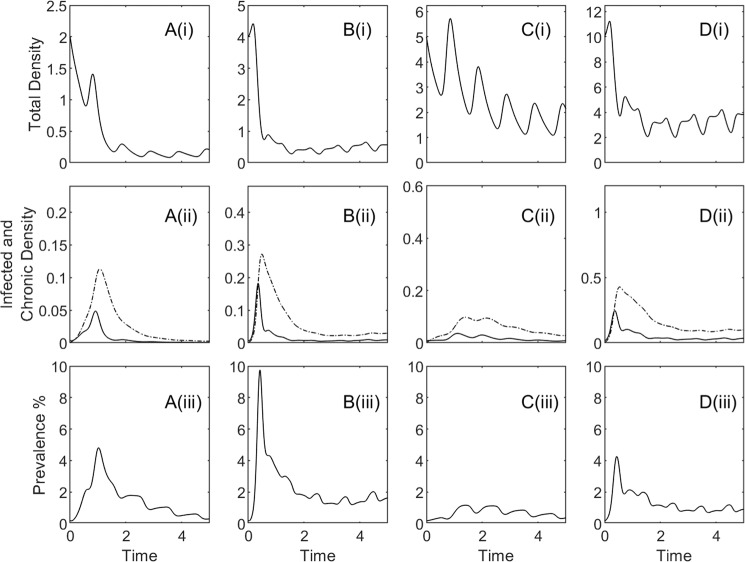
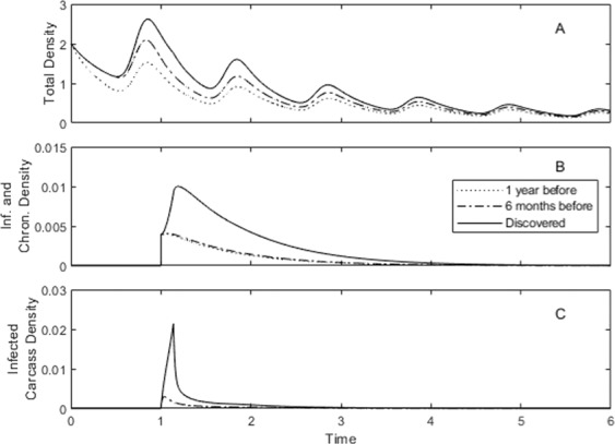
African swine fever (ASF) is a severe viral disease that is currently spreading among domestic pigs and wild boar (Sus scrofa) in large areas of Eurasia. Wild boar play a key role in the spread of ASF, yet despite their significance, little is known about the key mechanisms that drive infection transmission and disease persistence. A mathematical model of the wild boar ASF system is developed that captures the observed drop in population density, the peak in infected density and the persistence of the virus observed in ASF outbreaks. The model results provide insight into the key processes that drive the ASF dynamics and show that environmental transmission is a key mechanism determining the severity of an infectious outbreak and that direct frequency dependent transmission and transmission from individuals that survive initial ASF infection but eventually succumb to the disease are key for the long-term persistence of the virus. By considering scenarios representative of Estonia and Spain we show that faster degradation of carcasses in Spain, due to elevated temperature and abundant obligate scavengers, may reduce the severity of the infectious outbreak. Our results also suggest that the higher underlying host density and longer breeding season associated with supplementary feeding leads to a more pronounced epidemic outbreak and persistence of the disease in the long-term. The model is used to assess disease control measures and suggests that a combination of culling and infected carcass removal is the most effective method to eradicate the virus without also eradicating the host population, and that early implementation of these control measures will reduce infection levels whilst maintaining a higher host population density and in some situations prevent ASF from establishing in a population.

Figure 1

Population densities and prevalence over time for the model described by equations (1). All results were obtained using MATLAB software, specifically the built-in ODE solver packages. Total densities are given in (i), infected (solid line) and survivor (dashed line) densities in (ii), with prevalence, defined as I/N, in (iii). The plots in A and B represent the scenario for Estonia, under natural conditions and with supplementary feeding respectively. In C and D we show the model results for the scenario that represents Spain, under natural conditions and with supplementary feeding respectively. For Estonia we have d = 52/8, with K = 2 (A) and K = 4 (B). For Spain d = 52 with K = 5 (C) and K = 10 (D). Other parameters are β_F = 63, β_E = 2, ρ = 0.85, b_C = 0 and r = 0 (see also section S1).

Figure 2

Population response to a varying culling intensity, b_C, with three different carcass removal rates r = 0 (solid line), r = 26 (dashed) and r = 52 (dotted), for the model represented by equations (1). The total density, N, is given in A, with infected and survivor density in B and carcass density in C. Results are shown for the scenario that represents natural conditions in Estonia (see Fig. 1 for parameters) and show the average densities between the years 2 and 3 following disease introduction. Control measures were implemented as soon as the virus is first discovered, defined as the time when carcass levels first reach a density of 0.02. The value b_C corresponds to a culling proportion equal to $1-e^{-b_C}$, per year, of the total population.

Figure 3

Population response to a varying carcass removal rate, r, with three different culling intensities b_C = 0 (solid line), b_C = 0.75 (dashed) and b_C = 1.5 (dotted), for the model represented by equations (1). The total density, N, is given in A, with infected and survivor density in B and carcass density in C. Results are shown for the scenario that represents natural conditions in Estonia (see Fig. 1 for parameters) and show the average densities between the years 2 and 3 following disease introduction. Control measures were implemented as soon as the virus is first discovered, defined as the time when carcass levels first reach a density of 0.02. The value r corresponds to an average removal time, in years, of 1/r.

Figure 4

Population response to the combination of culling, at fixed rate b_C = 0.75, and carcass removal, at fixed rate r = 52, for the model represented by equations (1) and for parameters that represent the scenario in Estonia under natural conditions (see Fig. 1 for parameters).The total density, N, is given in A, with infected and survivor densities in B and prevalence in C. The results are shown for two different control implementation times: when the virus is first discovered (solid line), and six months after the virus was discovered (dashed line).

Figure 5

Population response to the combination of culling, at fixed rate b_C = 0.75, and carcass removal, at fixed rate r = 52, for the model represented by equations (1) and for parameters that represent the scenario in Estonia under natural conditions (see Fig. 1 for parameters).The total density, N, is given in A, with infected and survivor densities in B and prevalence in C. The results are shown for three different control implementation times: one year before the onset of the virus (dotted line), six months before the onset of the virus (dashed line), and when the virus is first discovered (solid line).

References

1. Gallardo MC, et al. African swine fever: a global view of the current challenge. Porcine Health Management. 2015;1:1–14. doi: 10.1186/s40813-015-0013-y. - DOI - PMC - PubMed
1. Korennoy FI, et al. Spatio-temporal modeling of the African swine fever epidemic in the Russian Federation, 2007–2012. Spatial and Spatiotemporal Epidemiology. 2014;11:135–141. doi: 10.1016/j.sste.2014.04.002. - DOI - PMC - PubMed
1. Simulundu E, et al. The Epidemiology of African Swine Fever in "Nonendemic” Regions of Zambia (1989–2015): Implications for Disease Prevention and Control. Viruses. 2017;9:1–20. doi: 10.3390/v9090236. - DOI - PMC - PubMed
1. Vergne T, Korennoy F, Combelles L, Gogin A, Pfeiffer DU. Modelling African swine fever presence and reported abundance in the Russian Federation using national surveillance data from 2007 to 2014. Spatial and Spatio-temporal Epidemiology. 2016;19:70–77. doi: 10.1016/j.sste.2016.06.002. - DOI - PubMed
1. Depner, K. et al. Scientific report on the epidemiological analyses of African swine fever in the Baltic States and Poland. European Food Safety Authority Journal 15, 1–59 (2017). - PMC - PubMed
Publication types