The shape of things to come: Topological data analysis and biology, from molecules to organisms

Abstract

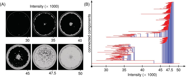
Shape is data and data is shape. Biologists are accustomed to thinking about how the shape of biomolecules, cells, tissues, and organisms arise from the effects of genetics, development, and the environment. Less often do we consider that data itself has shape and structure, or that it is possible to measure the shape of data and analyze it. Here, we review applications of topological data analysis (TDA) to biology in a way accessible to biologists and applied mathematicians alike. TDA uses principles from algebraic topology to comprehensively measure shape in data sets. Using a function that relates the similarity of data points to each other, we can monitor the evolution of topological features-connected components, loops, and voids. This evolution, a topological signature, concisely summarizes large, complex data sets. We first provide a TDA primer for biologists before exploring the use of TDA across biological sub-disciplines, spanning structural biology, molecular biology, evolution, and development. We end by comparing and contrasting different TDA approaches and the potential for their use in biology. The vision of TDA, that data are shape and shape is data, will be relevant as biology transitions into a data-driven era where the meaningful interpretation of large data sets is a limiting factor.

Keywords: biology; data science; mathematical biology; persistent homology; shape; topological data analysis.

FIGURE 1

An example of geometric morphometrics. A, 24 landmarks (orange dots) and pseudo‐landmarks (6000 evenly spaced vertices between landmarks, magenta dots) on grapevine leaves of Cabernet sauvignon (orange), Chardonnay (blue), and Chasselas cioutat (green) varieties. Every grapevine leaf has five major veins, allowing corresponding landmarks to be placed throughout every leaf. B, Corresponding vertices allow replicates to be superimposed on each other, and C, mean leaves calculated using Procrustean methods that translate, rotate, reflect, and scale. D, A principal component analysis (PCA) and other statistics can be performed on the Procrustes‐adjusted vertices (95% confidence ellipses for each variety are shown)

FIGURE 2

An example of a complex. It has two connected components, one loop, and one void

FIGURE 3

An example of two different Vietoris‐Rips complexes with resulting persistence barcodes. A, Evolution of a VR complex with five vertices as Euclidean distance increases. B, Persistence barcode corresponding to topological changes in the previous VR complex. C, Alternative visualization of the persistence of barcode B as a dendrogram. D, Alternative visualization of the persistence of barcode B as a tree. E, Moving one vertex in A yields a different VR complex as Euclidean distance increases. F, Persistence barcode corresponding to topological changes in the previous complex E. G, Alternative visualization of the persistence barcode F as a dendrogram. H, Alternative visualization of the persistence barcode F as a tree

FIGURE 4

Translating a persistence barcode into a persistence diagram. Birth and death times in the persistence barcode are interpreted as x‐y coordinates on a death‐vs‐birth plane. This planar display is referred to as a persistence diagram

FIGURE 5

An example of a persistence barcode. A, Snapshots of an X‐ray CT image of an orange. Only the pixels with intensity lower than indicated are displayed. B, Persistence barcode of connected components of such an image. Observe that the barcode distinguishes the existence of exocarp, rind, and pith as separate components at lower intensities

FIGURE 6

Applications of topological data analysis (TDA) to biology. A, Structural biology. A diagram of RNA secondary structure (left; solid lines covalent bonds, dashed lines hydrogen bonds). Increasing radii of vertices (middle, right; blue points) are used to visualize filtration on Euclidean distance. As radii merge, connected components die. Purple lines indicate the formation of loops that eventually fill in as the radius threshold increases. B, Evolution. A plot showing the genetic distance of samples (left). As radius threshold value increases (middle, right) the birth and death of connected components (blue) represent vertical evolution (a tree) while that of loops (purple) horizontal evolution events (such as hybridization, gene transfer, or recombination; modified from Reference 13). C, Cellular architecture. Modification of a part of the original Gleason guide to prostate cancer changes in cellular architecture (left). Nuclei (blue) increase in radius (middle, right) and connected components (blue) and loops (purple) are born and die. D, Branching architecture. A theoretical tree where the filter is the geodesic distance to the base (blue). Branching tips are separate connected components that merge as the filter progresses to the base of the tree (left to right). E, Mapper. Point cloud of a hand where the filter is the axes from the wrist to fingertips (left). Cover intervals (bars on top of the color scale) and their overlap (gray bars) divide points into bins (middle). Points that cluster together over each cluster are assigned to a vertex, and if the points are shared between clusters in an overlap, then they are assigned to an edge connecting the corresponding vertices (modified from Reference 42)

FIGURE 7

Three different Euler characteristic curves (ECCs) from three different filters. A, X‐ray CT scan of a barley seed. The symmetry of the seed encourages a filter by depth, width, and height values, that is, the three main axis directions with respect to the seed scan. Slicing the barley seed in different directions produce, B, different corresponding ECCs. Notice that the three curves end with Euler characteristic equal to one, which corresponds to the Euler characteristic of a solid sphere

FIGURE 8

Computing the bottleneck distance between two persistence diagrams. A, A possible pairing of points is suggested. Observe that it produces a large maximum distance between pairs. B, An alternate pairing that yields a considerably smaller maximum distance between pairs

FIGURE 9

An example of mapper graphs. A, X‐Ray CT scan of a gall filtered by distance from the center. B, These filter values are projected to a real line. The real line is then covered by a collection of overlapping intervals. For each interval, we then form different clusters of voxels whose filter value is in such interval. These clusters then yield the vertices and edges of, C, a mapper graph. Formally, the vertices are connected components within a certain range of radius from the center and edges correspond to overlap. Size of vertices and edges corresponds to the size of the component or overlap

FIGURE 10

Endless forms most beautiful. X‐ray Computed Tomography (CT) scans of biological specimens showing the diversity of morphology in the natural world. A, Magnolia bud, B, bean flowers, C, grapevine leaf with phylloxera galls, D, the fasciated meristem of a velvet flower, E, side view of a sunflower disc, F, bell pepper, G, tree rings, H, marigold flower, I, vasculature within an apple, J, Haworthia, K, Echeveria, L, Agave hybrid, M, citrus fruit, N, monkeyflower, O, archaeological sunflower disc specimen

References

1. Bookstein FL. Morphometric Tools for Landmark Data: Geometry and Biology. Cambridge: Cambridge University Press; 1997.
1. Gower JC. Generalized procrustes analysis. Psychometrika. 1975;40:33‐51. 10.1007/BF02291478. - DOI
1. Lestrel Pete E. (editor). Fourier Descriptors and their Applications in Biology. Cambridge: Cambridge University Press; 1997. doi: 10.1017/CBO9780511529870 - DOI
1. Kuhl FP, Giardina CR. Elliptic Fourier features of a closed contour. Comput Graph Image Proc. 1982;18(3):236‐258. 10.1016/0146-664X(82)90034-X. - DOI
1. Chitwood DH, Sinha NR. Evolutionary and environmental forces sculpting leaf development. Curr Biol. 2016;26(7):R297‐R306. 10.1016/j.cub.2016.02.033. - DOI - PubMed
Publication types
LinkOut - more resources