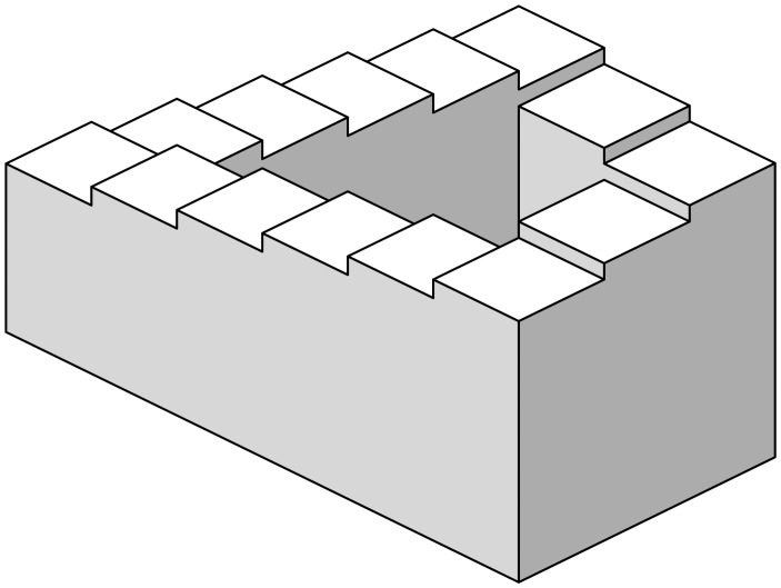
Climbing Escher's stairs: A way to approximate stability landscapes in multidimensional systems

Abstract

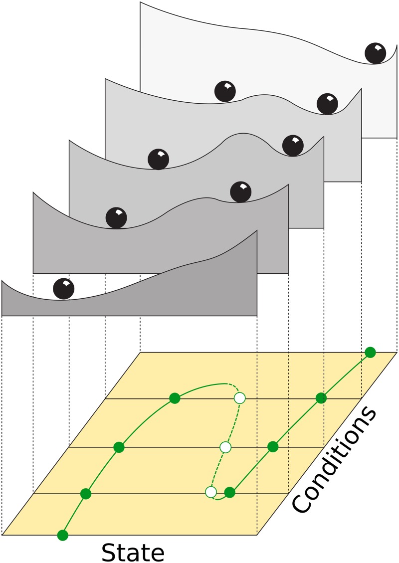
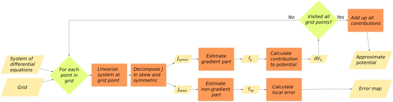
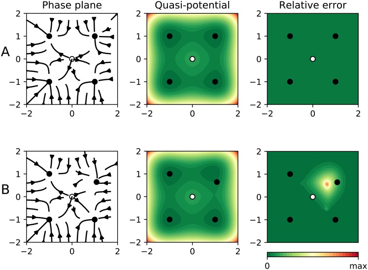
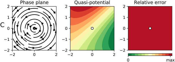
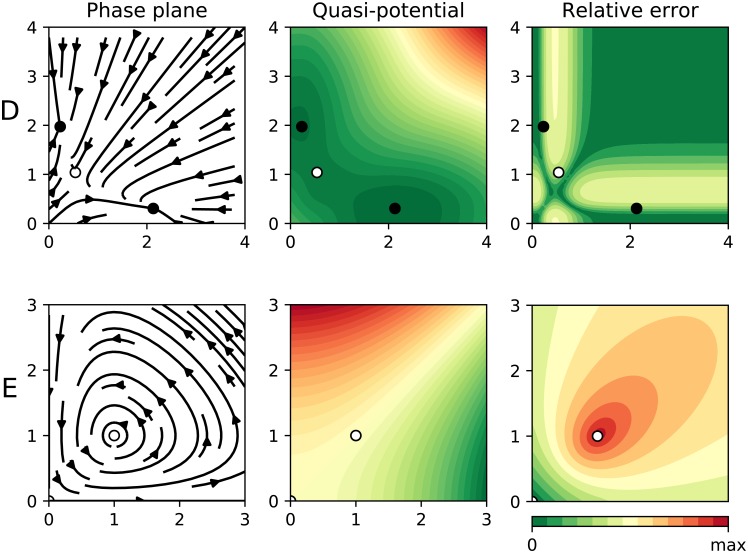
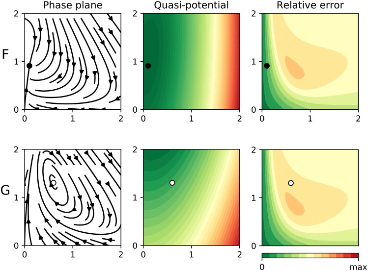
Stability landscapes are useful for understanding the properties of dynamical systems. These landscapes can be calculated from the system's dynamical equations using the physical concept of scalar potential. Unfortunately, it is well known that for most systems with two or more state variables such potentials do not exist. Here we use an analogy with art to provide an accessible explanation of why this happens and briefly review some of the possible alternatives. Additionally, we introduce a novel and simple computational tool that implements one of those solutions: the decomposition of the differential equations into a gradient term, that has an associated potential, and a non-gradient term, that lacks it. In regions of the state space where the magnitude of the non-gradient term is small compared to the gradient part, we use the gradient term to approximate the potential as quasi-potential. The non-gradient to gradient ratio can be used to estimate the local error introduced by our approximation. Both the algorithm and a ready-to-use implementation in the form of an R package are provided.

Fig 1. Example of a set of 5 stability landscapes used to illustrate bistability in ecosystems (e.g: Forest/Desert, eutrophicated lake/clear water, etc., see [7]).

The upper side of the figure shows the stability landscape of a one-dimensional system for 5 different values of a control parameter. The lower side shows the bifurcation diagram, where the filled points represent stable equilibria and the empty points unstable ones. This diagram proved to be a successful tool for explaining advanced concepts in dynamical systems theory such as bistability and fold bifurcations to scientific communities as diverse as ecologists, mathematicians and environmental scientists.

Fig 2. The Penrose stair [8] is a classical example of an impossible object.

In such a surface, it is possible to walk in a closed loop while permanently going downhill. The scalar potential of a system with a cyclic attractor, if existed, should have the same impossible geometry. This object was popularized by the Dutch artist M.C. Escher (for two beautiful examples, see [9] and [10]).

Fig 3. Flowchart showing the basic functioning of our implementation of the algorithm described in this paper.

Fig 4. Results for two synthetic examples.

In all panels the dots represent equilibrium points (black for stable, otherwise white). The left panel shows the phase plane containing the actual “deterministic skeleton” of the system. The central panel shows the quasi-potential. The right panel shows the estimated error. Row A shows the application to a gradient case (Eq (20) with interaction terms equal to zero). As expected, the error is zero everywhere. In row B our algorithm is applied to a non-gradient case (Eq (20), with non-zero interaction terms).

Fig 5. Results for a fully non-gradient system (Eq (21)).

In all panels the dots represent center equilibrium points. The left panel shows the phase plane containing the actual “deterministic skeleton” of the system. The central panel shows the quasi-potential. The right panel shows the estimated error.

Fig 6. Results for two biological systems.

In all panels the dots represent equilibrium points (black for stable, otherwise white). The left panel shows the phase plane containing the actual “deterministic skeleton” of the system. The central panel shows the quasi-potential. The right panel shows the estimated error. In row D we applied our algorithm to the simple gene regulatory network described in Eq (22). In row E we apply our algorithm to a Lotka-Volterra system (Eq (23), with a = b = c = d = 1).

Fig 7. Results for two parameter settings of the Selkov model (Eq (24)).

In all panels the dots represent equilibrium points (black for stable, otherwise white). The left panel shows the phase plane containing the actual “deterministic skeleton” of the system. The central panel shows the quasi-potential. The right panel shows the estimated error. In row F we applied our algorithm to a Selkov system with b = 0.1, so the solutions reach a stable point. In row G we set b = 0.6, so the system has a limit cycle.

References

-
- Edelstein-Keshet L. Mathematical Models in Biology [Internet]. Society for Industrial; Applied Mathematics; 1988.
- Strogatz SH. Nonlinear Dynamics And Chaos: With Applications To Physics, Biology, Chemistry And Engineering. 1994. p. 512.
- Beisner B, Haydon D, Cuddington K. Alternative stable states in ecology Frontiers in Ecology and the Environment. John Wiley & Sons, Ltd; 2003;1: 376–382.
Publication types
MeSH terms
LinkOut - more resources
Full Text Sources