The natverse, a versatile toolbox for combining and analysing neuroanatomical data

Abstract

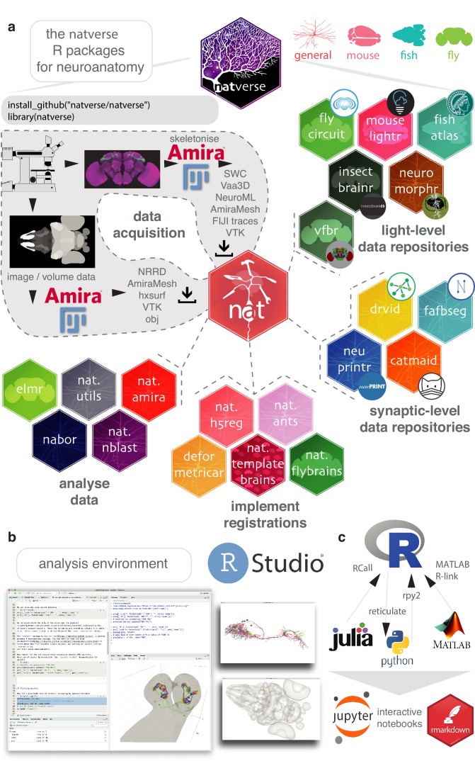
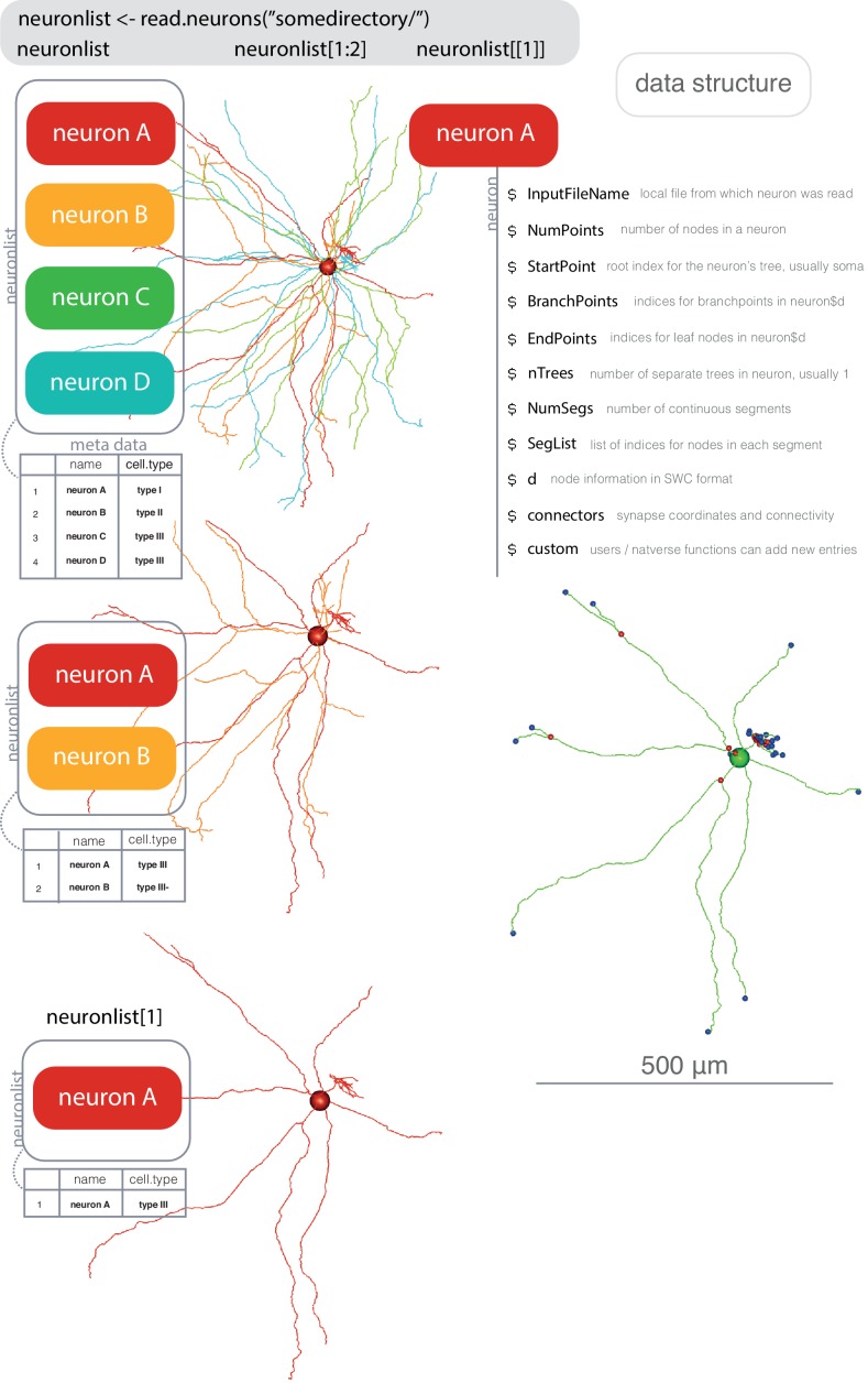
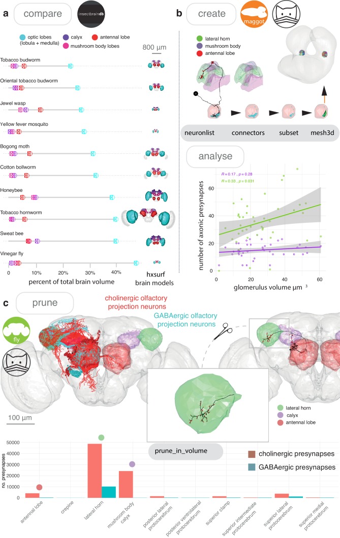
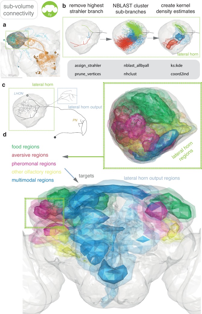
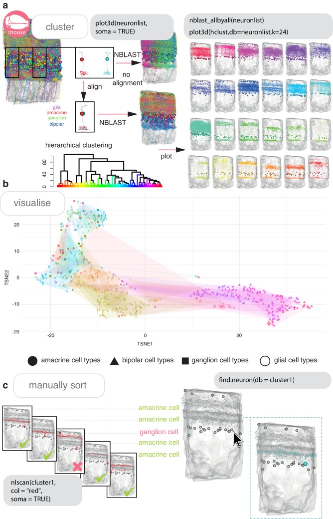
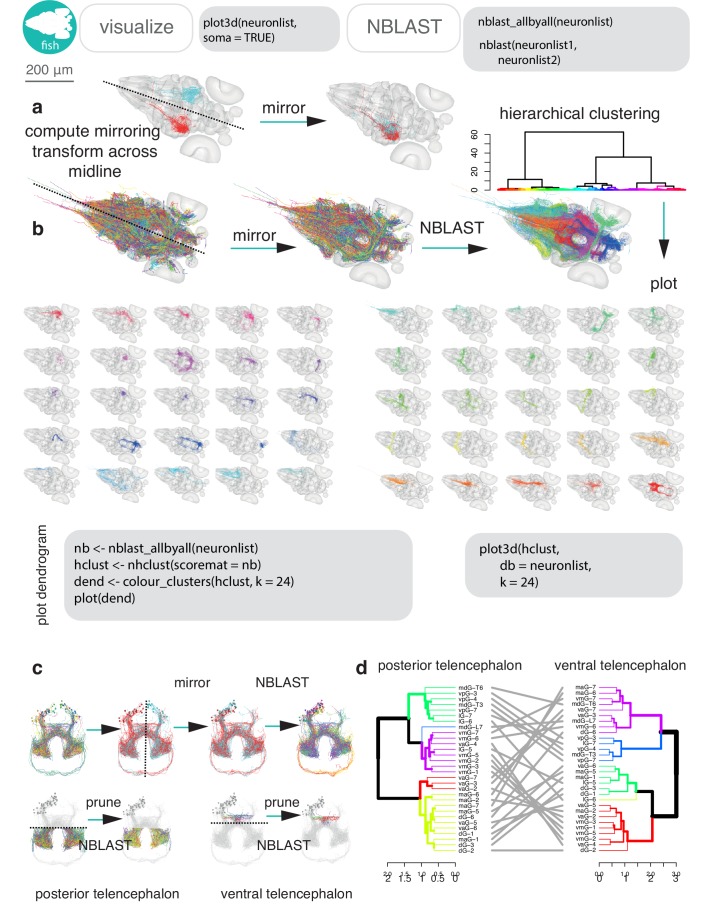
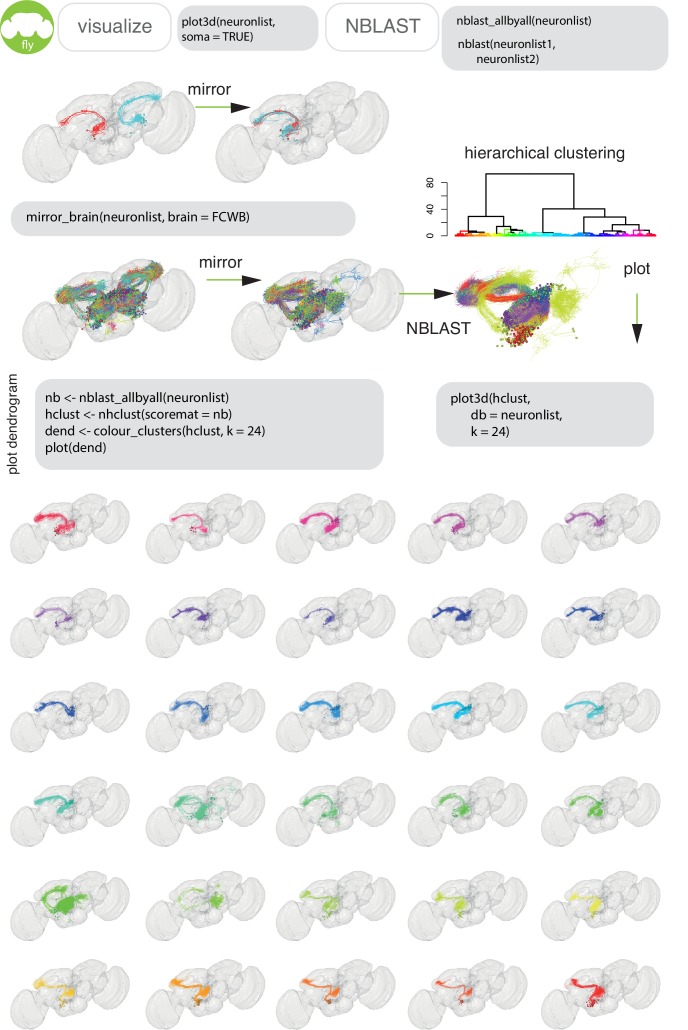
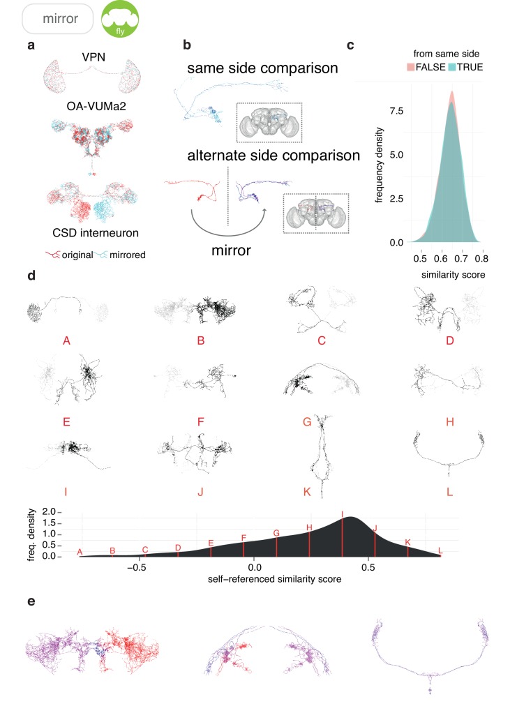
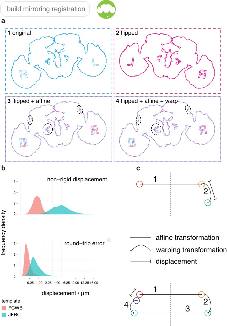
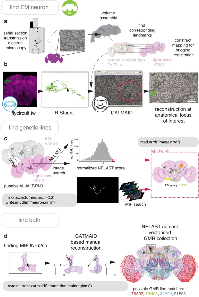
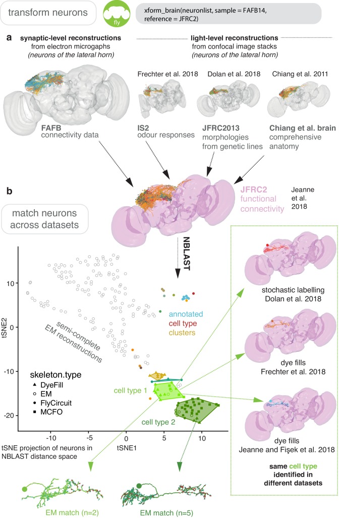
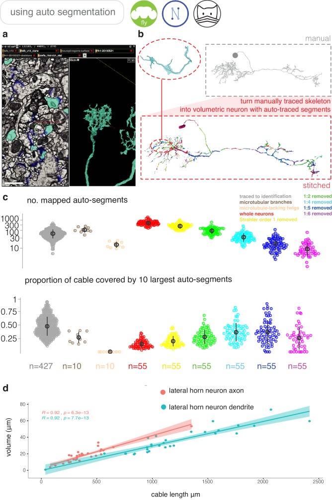
To analyse neuron data at scale, neuroscientists expend substantial effort reading documentation, installing dependencies and moving between analysis and visualisation environments. To facilitate this, we have developed a suite of interoperable open-source R packages called the <monospace>natverse</monospace>. The <monospace>natverse</monospace> allows users to read local and remote data, perform popular analyses including visualisation and clustering and graph-theoretic analysis of neuronal branching. Unlike most tools, the <monospace>natverse</monospace> enables comparison across many neurons of morphology and connectivity after imaging or co-registration within a common template space. The <monospace>natverse</monospace> also enables transformations between different template spaces and imaging modalities. We demonstrate tools that integrate the vast majority of Drosophila neuroanatomical light microscopy and electron microscopy connectomic datasets. The <monospace>natverse</monospace> is an easy-to-use environment for neuroscientists to solve complex, large-scale analysis challenges as well as an open platform to create new code and packages to share with the community.

Keywords: D. melanogaster; analysis software; computational biology; connectomics; mouse; neural circuits; neuroanatomy; neuronal morphology; neuroscience; open-source; systems biology; zebrafish.

Figure 1.. The natverse.

(a) R packages that constitute the natverse. Packages are coloured by whether they are general purpose, or cater specifically for Mus musculus, Danio rerio or Drosophila melanogaster datasets. Coarse division into packages for fetching remote data, implementing registrations and analysing data are shown. Data, as outputted by most reconstruction pipelines, can also be read by nat. (b) The natverse is designed to work best in the RStudio environment (RStudio Team, 2015), by far the most popular environment in which to execute and write R code. 3D visualisation is based on the R package rgl (Murdoch, 2001), which is based on OpenGL and uses the XQuartz windowing system. It runs on Mac, Linux and Windows platforms. (c) R functions can be called by other popular scientific programming languages, some example packages/libraries are shown. In particular, there is support for bidirectional interaction with Python, with interactive use supported by Jupyter or R Markdown notebooks. One of us (P. Schlegel) has developed Python code inspired by the natverse for analysing neuron morphology, NAVIS (https://github.com/schlegelp/navis), and talking to the CATMAID API, PyMaid (https://github.com/schlegelp/pyMaid). These python libraries transform natverse-specific R objects into Python data types and can call natverse R functions like nblast.

Figure 1—figure supplement 1.. A basic analysis pipeline.

A simple pipeline for neuron analysis with nat. Bouton placement for a layer 5 pyramidal neuron from the mouse primary somatosensory cortex is examined relative to the neuron’s cable length and position within the layered structure of the cortex. Coloured names indicate layer transitions. Data courtesy of A. Vourvoukelis, A. von Klemperer and C.J. Akerman.

Figure 2.. Neurons in nat.

(a) Data classes defined by nat. A D. melanogaster DA1 olfactory projection neuron (Costa et al., 2016) is shown as part of four different data types, useful for different sorts of analyses: as a neuron object (left), as part of a larger neuronlist of multiple olfactory projection neurons (middle), as a vector-cloud dotprops object (right, upper) and a ngraph object (right, lower). In grey, the FCWB template brain, a hxsurf object from the package nat.flybrains, is shown. Generic code for visualizing these data types shown. (b) Visualisation, with generic sample code, of connectomic data from a dense reconstruction inner plexiform layer of the mouse retina is shown, coloured by the cell class and then cell type annotations given by their reconstructors (Helmstaedter et al., 2013). Because this dataset contains many neuron fragments that have been severely transected, we only consider skeletons of a total cable length greater than 500 μm using functions summary and subset. Somata are shown as spheres. (c) A synaptic-resolution neuron reconstruction for a D. melanogaster lateral horn neuron (Dolan et al., 2018a) has been read from a live CATMAID project hosted by Virtual Fly Brain (https://fafb.catmaid.virtualflybrain.org/) using catmaid, and plotted as a neuron object. It is rooted at the soma, consistent with the convention. (d) Boxed, Strahler order is a measure of branching complexity for which high Strahler order branches are more central to a neuron’s tree structure, and the lower order ones more peripheral, such that branches with leaf nodes are all Strahler order 1. Main, the same neuron which has had its lower Strahler order branches (see inset) progressively pruned away. (e) We can extract the longest path through a neuron, its ‘spine’, purple, a method that could help define the tracts that a neuron might traverse. (f) Boxed, in insect neurons, the main structure of the neuron is supported by a microtubular backbone. As it branches its more tortuous, smaller caliber neurites loose the microtubule, and make more postsynapses (Schneider-Mizell et al., 2016). Main, in CATMAID users can tagged the tree nodes that mark the position where neurite loses its microtubular backbone, so an R user can use prune family functions to remove, add or differentially colour microtubular backbone versus twigs. (g) Both presynapses and postsynapses can been manually annotated in CATMAID, and be visualised in R. Because neurons from CATMAID have synaptic data, they are treated as a slightly different class by the natverse, called catmaidneuron. A neuronlist can also comprise many catmaidneuron objects. (h) Right, using synaptic information, it is possible to use a graph theoretic approach which divides the neuron at the point of maximum ‘flow’ - the region in the neuron at which there are the most parallel paths - having ‘drawn’ a path between each input synapse and each output synapse that pass through every node on the skeleton (Schneider-Mizell et al., 2016). This helps divide a neuron into its dendrites, axon, intervening cable (maximum flow, the primary dendrite) and its cell body fiber (no flow). In insects, the cell body lies outside the neuropil and is connected to its arbour by a single fiber. Main, axon-dendrite split shown for exemplary neuron using seesplit3d.

Figure 2—figure supplement 1.. Neurogeometry and skeleton annotations with nat.

(a) We used neuromorphr to obtain information about 40599 mammalian neurons from NeuroMorpho.org, in the brain region ‘neocortex’, from 193 different laboratories. However, it is quite difficult to compare morphologies acquired from different laboratories, that have used different imaging pipelines, neuron reconstruction tools and staining protocols (Farhoodi et al., 2019). We can use neuromorphr to access neuron metadata on NeuroMorpho.org, and choose only those neurons from the same laboratory (Bob Jacobs’), that have been obtained using a Golgi stain and the reconstruction software NeuroLucida, and that are classed as a principal cell (Anderson et al., 2010; Anderson et al., 2009; Jacobs et al. (2018); Jacobs et al., 2016; Jacobs et al., 2015; Jacobs et al., 2011; Jacobs et al., 2001; Jacobs et al., 1997; Reyes et al. (2016); Travis et al., 2005), giving us 3174 neurons. Branch points per micron cable can then be plotted for 24 different species’ cortical principal neurons using ggplot2. (b) Inset, a Sholl analysis (Sholl, 1953) obtains the number of intersections the neurons’ morphologies make with radii of increasing size centered at their roots. Main, the mean intersections for a subset of the species’ cortical principal cells is shown. (c) The distribution of pre- and post-synapses along three neurons arbors, split by axon and dendrite, then further by Strahler order, then further by presence (backbone) or absence (twigs) of microtubule. Olfactory related neurons (gold), associative memory related neurons (purple) and unknown inputs (grey). In this case, neuron#1 and neuron#2 are of the same cell type and look similar (PD2a1), but neuron#3 differs, indeed it belongs to a different cell type (PD2b1) (Dolan et al., 2018a).

Figure 2—figure supplement 2.. Neuron data structure.

Schematic representation of the data structure behind neuron objects and neuronlist objects. Objects of class neuronlist are essentially lists of neuron objects, representing one or more neurons, with some attached metadata.

Figure 3.. Neuroanatomical models with nat.

(a) We accessed the InsectBrainDB.org via insectbrainr to obtain template brains for different species of insect (Brandt et al., 2005; de Vries et al., 2017; El Jundi et al., 2018; Heinze and Reppert (2012); Kurylas et al. (2008); Løfaldli et al. (2010); Stone et al. (2017); Zhao et al., 2014). The package insectbrainr converts retrieved OBJ files into hxsurf objects, which contain one set of 3D points for each whole brain, and then different sets of edges between these points to form 3D neuropil subvolumes. These subvolumes were already defined by expert annotators. Their volume are compared across insect brain, normalised by total brain size. Insect template brain data curated by: S. Heinze, M. Younger, J. Rybak, G. Pfuhl, B. Berg, B. el Jundi, J. Groothuis and U. Homberg. (b) We can create our own subvolumes by pulling synaptic neuron reconstructions (Berck et al., 2016) from a first-instar larva EM dataset (Ohyama et al., 2015) (a public CATMAID instance hosted by Virtual Fly Brain), extracting dendritic post synapses from olfactory projections neurons, and using synapse clouds from neurons of the same cell type, to define glomerular volumes by creating a bounding volume, i.e an α-shape or convex hull. Their volumes can then be calculated, and correlated with the number of presynapses the same neurons make in two higher-order brain regions, the lateral horn and the mushroom body calyx. (c) Volumes can be used to analyse skeleton data. In (c) we look again at olfactory projection neurons, this time from an adult fly EM dataset (Zheng et al., 2018) and use the nat function pointsinside with standard neuropil volumes (Ito et al., 2014) to find the numbers of presynapses GABAergic and cholinergic olfactory projection neurons from the antennal lobe make in different neuropils. These neuropils exist as a hxsurf object in our R package nat.flybrains.

Figure 3—figure supplement 1.. Superxovel analysis with nat.

(a) The basic connectivity scheme of the lateral horn, a second order olfactory centre in insects. Olfactory projection neurons (in orange) connect to lateral horn neurons (in cyan) (Frechter et al., 2019). (b) To create anatomically meaningful continuous voxels for the lateral horn, rather than random contiguous partitions of our standard neuropil space (Ito et al., 2014), we first removed the highest Strahler order branch (assign_strahler) from projection neuron axons’ so that their sub-branches could be clustered into 25 separate groups (nblast). For each cluster, a 3-D weighted kernel density estimate was generated based on 3D points (xyzmatrix) extracted from clustered sub-branches, using the R package ks (Duong, 2007). Points were spaced on neurites at 1 μm intervals (resample) and weighted as 1/total number of points in the cluster, so that supervoxels could be directly compared. (c) An 'inclusion' score for each neuron was calculated for each supervoxel by summing the density estimate for each point in the chosen arbor, again sampled at 1 μm intervals, and normalised by the total number of points in each arbor. An atlas of the lateral horn, colouring supervoxels by the modality/valence of their strongest input neurons. (d) A ‘projection’ was calculated between each lateral horn voxel and each lateral horn output voxel based on the number of neuronal cell types that have processes in both and the density of this arborisation. An atlas of the lateral horn output regions can then be made, colouring supervoxels by the modality/valence of their strongest input lateral horn supervoxels.

Figure 4.. Cell typing with nat.

(a) Neurons from a dense reconstruction from EM data of the mouse retina inner plexiform layer (Helmstaedter et al., 2013) can either be NBLAST-ed in situ (upper) or after alignment by their principal axes in 3D space (lower) in order to make a first pass at defining, finding or discovering morphological neuronal cell types using NBLAST. (b) A tSNE plot visualising the results of an aligned NBLAST of neurons in A, coloured by the manually annotated cells types seen in Figure 2c, with shapes indicating the cell class. (c) Manual sorting using the interactive nat functions nlscan and find.soma or find.neuron can help identify misclassifications and make assignments.

Figure 4—figure supplement 1.. Cell typing zebrafish neurons with nat.

(a) Light-level neurons registered to a standard brain for the larval zebrafish (Kunst et al., 2019) can be read into R using fishatlas, and all transformed onto the right hemisphere using the mirroring registration generated by Kunst et al. (b) They can then be NBLAST-ed to discover new cell types. 25 NBLAST clusters are shown, generic exemplary code shown in Monaco font. (c) Upper, shows this process for a small group of neurons from the telencephalon. Mirroring neurons to the same side produces cohesive clusters. Lower, neurons can be cut up (pruned) relative to user defined coordinates to, in this case, divide them by telencephalon region. NBLAST can be run separately on these two groups, and the results were compared using a tanglegram to see whether neurons that cluster together in the posterior telencephalon, also cluster together in the ventral telencephalon.

Figure 4—figure supplement 2.. Cell typing vinegar fly neurons with nat.

The same basic process can be done for FlyCircuit neurons (Chiang et al., 2011), here subsetted (in_volume) to those neurons that have arbor in both the antennal lobe and lateral horn (i.e. olfactory projection neurons).

Figure 5.. Sample applications of mirroring registrations.

(a) Three FlyCircuit neurons along with mirrored versions; a visual projection neuron, OA-VUMa2 (Busch et al., 2009) and the CSD interneuron (Dacks et al., 2006). Co-visualisation facilitates the detection of differences in innervation, such as the higher density of innervation for the CSD interneuron in the lateral horn on the contralateral side compared to the ipsilateral lateral horn. (b) Neurons from the same side of the brain and alternate side of brain are compared and a similarity score generated. (c) Distributions of similarity scores for comparisons within the same brain hemisphere and across brain hemispheres. These scores are similar, because the mirroring registration is good. (d) Sequence of 12 example neurons (black) with mirrored counterparts (grey), having equally spaced similarity scores. Below, full distribution of scores for all neurons in FlyCircuit dataset. (e) Segment-by-segment measures of neuron similarity. Redder shades correspond to low degrees of symmetricity, bluer shades higher. Flipped version of neuron in gray.

Figure 5—figure supplement 1.. Mirroring procedure.

(a) The full process undergone by an image during a mirroring registration. (1) Original image. (2) Flipped 180° around the medio-lateral axis. (3) Affinely transformed. (4) Non-rigidly warped. (b) Heatmaps of deformation magnitude fields for mirroring FlyCircuit and FlyLight reference brains. (c) Distribution of deformation displacements for both brains, in a single mirroring operation and a full round-trip. Illustrations show the transformations that points undergo.

Figure 6.. Bridging registrations for brain templates.

(a) A small sample of Drosophila template brains used around the world are shown. (b) A partial neuron tracing (purple) made using Simple Neurite Tracer (Longair et al., 2011) being transformed (xform_brain) from the IS2 standard brainspace to the FCWB, where it can be co-visualised with a more complete, matching morphology from FlyCircuit, using our R package flycircuit. (c) Outermost neuropil boundaries for FlyCircuit (red) and FlyLight (cyan) template brains. Primed space names indicate original spaces for data. Unprimed space names indicate current space of image. (d) Neuropil segmentation from JFRC2 space alongside FCWB reformatted version. (e) CSD interneuron from FlyCircuit (red) and FlyLight, GMR GAL4 expression pattern (cyan). (f) Neuropil segmentation from JFRC2 (Ito et al., 2014) space that has been bridged into FCWB space, so it can be seen along with selected neurons from FlyCircuit. (g) A traced neuron in FCWB space alongside morphologically similar neuron from FlyCircuit. (h) Expression pattern of Vienna Tiles line superimposed on expression pattern of FlyLight line. (Since we made our bridging publically available in April 2014, Otsuna et al., 2018 have also, separately, bridged these two datasets.).

Figure 6—figure supplement 1.. Bridging procedure.

(a) Increasing levels of registration complexity give increasingly good registration results. (b) Four composite transformations of a 12-degree-of-freedom affine transformation. (c) Regularly spaced grid of control points (red dots) in the reference brain. (d) Control points (cyan dots) in the sample image. (e) Sample brain control points affinely transformed into image space of reference brain, along with original control points. (f) Deformation field interpolated using B-splines. (g) Reformatted sample image.

Figure 6—figure supplement 2.. Bridging examples.

(a) A sub-section of the bridging registrations available through nat.flybrains, via which a neuroanatomical entity in any brainspace can eventually be placed into any other brainspace, by chaining bridging registrations. Arrows indicate the existence and direction of a bridging registration. Registrationfrye@ucla.edus are numerically invertible and can be concatenated, meaning that the graph can be traversed in all directions. Both brains (Arganda-Carreras et al., 2018; Bogovic et al., 2018; Cachero et al., 2010; Costa et al., 2016; Ito et al., 2014; Jefferis et al., 2007; Jenett et al., 2012; Rein et al., 2002; Tirian and Dickson, 2017; Zheng et al., 2018) and ventral nervous systems (Cachero et al., 2010; Yu et al., 2010) shown. (b) Fru+ neuroblast clones (orange) transformed from IS2 space into JFRC2 space of elav neuroblast clones (green). (c) Sexually dimorphic Fru+ neuroblast clone (male on left, female on right) along with traced neurons from FlyCircuit.

Figure 6—figure supplement 3.. Warping registration without point-point correspondence.

(a) A left-right registration for the lop-sided nascent L1 larval connectome (Ohyama et al., 2015). Neuroanatomical models created from CATMAID data (upper) and 644 manually left-right paired neurons can be used as a basis to generate a single deformation of L1 space using Deformetrica (via deformetricar), that describes a left-right mapping in a single deformation of ambient space. (b) Symmetrisation (purple) of the lop-sided cortex and neuropil in the L1 EM dataset. (c) Registration of segmented light-level volumes onto the EM dataset. Immunohistochemical staining of dissected L1 central nervous system was needed to make 3D models for coarse neuroanatomical volumes, which could be matched to those in the L1 EM; namely, the pattern of longitudinal ventral nervous system axon tracts and the mushroom bodies, visible in a dFasciculin-II-GFP protein trap line, the laddered ventral nervous system pattern and olfactory tracts visible in a GH146-lexA line, and a Discs large-1/dN-Cadherin stain to visualize the neuropil and cortex of the brain.

Figure 7.. Finding specific neurons in EM and LM data.

(a) Pipeline for acquiring EM neuron data. Serial section transmission EM at high speed with a TEM camera array (Bock et al., 2011) produced several micrographs per section at 4 × 4 nm resolution, ~40 nm thick. These were, per section, stitched into mosaics which were, across sections, registered to create the female adult fly brain v.14 template space (FAFB14, grey) (Zheng et al., 2018). Corresponding landmarks between FAFB14 and JFRC2 can be found and used to build a bridge. (b) The R package elmr can be used to select an anatomical locus, here the PD2 primary neurite tract (Frechter et al., 2019), from 3D plotted light-level neurons, taken from FlyCircuit, and generate a URL that specifies its correct coordinates in a FAFB14 CATMAID instance. Candidates (185) may then be coarsely traced out until they deviate from the expected light-level morphologies (178 pink dotted profiles, often a few minutes to an hour of manual reconstruction time to rule out neurons of dissimilar cell types sharing a given tract, similar cell types are more subtly different and might need to be near completely reconstructed). Those that remain largely consistent were fully reconstructed (green profiles, ~7–12 person-hours per neuron) (Li et al., 2019). (c) Close matches reveal likely morphology of non-reconstructed branches (orange arrow) but also contain off-target expression (yellow arrow). Identification of multiple candidate lines enables split-GAL4 line generation aimed at retaining common neurons in two GAL4 patterns. MultiColor FlpOut (MCFO) (Nern et al., 2015) of resultant splits can be compared with the EM morphology. Here, a candidate GAL4 line is found for AL-lALT-PN3 (Frechter et al., 2019; Tanaka et al., 2012) using NBLAST and a MIP search (Otsuna et al., 2018). (d) A recent dense, but volume-restricted reconstruction of the mushroom body α-lobe discovered a ‘new’ mushroom body output neuron type (MBON-α2sp) (Takemura et al., 2017). By bridging from the correct mushroom-body compartment using a mushroom body mesh (Ito et al., 2014) visualised in R Studio, to the FAFB14 EM data’s equivalent space in CATMAID using the R package elmr, an experienced tracer can easily identify dendrites and find MBON-α2sp. By doing so, we found its previously unreported axon-morphology. We then imported the skeleton into R studio, bridged MBON-α2sp into the JFRC2 template space where it could be NBLAST-ed against GMR GAL4 lines to identify candidate lines containing the MBON.

Figure 8.. Bridging EM and LM data.

(a) Sparse EM reconstruction providing a database of non-comprehensive, partial morphologies that can be searched using NBLAST. Candidate neurons from the EM brainspace can be NBLAST-ed against MCFO (Nern et al., 2015) data and other light-level datasets in order to connect them to cell-type-specific information, such as odour responses and functional connectivity (Chiang et al., 2011; Dolan et al., 2019; Frechter et al., 2019; Jeanne et al., 2018), by bridging these datasets into the same brainspace. (b) An all-by-all NBLAST of all neurons in the PD2 primary neurite cluster (Frechter et al., 2019) in multiple datasets can be shown as a tSNE plot. EM cell type matches can easily be found, as well as other correspondences between the light level datasets.

Figure 8—figure supplement 1.. Using partial automatic segmentation of EM data.

(a) A NeuroGlancer window open on a web browser, showing an example of an automatic reconstruction. (b) Automatically reconstructed segments can be mapped onto extant manual tracing in FAFB14 using our R package fafbseg, enabling easy volumetric reconstruction of neurons. (c) Upper, automatically traced segments are mapped onto 55 manually reconstructed neurons from the lateral horn of D. melanogaster in the FAFB14 dataset (Bates et al., 2020), broken down by Strahler order, to simulate different levels of ‘completeness’. A further 10 neurons have had microtubular cable annotated. Lower, proportion of cable at different levels of pruning, that are covered by the 10 largest auto-segmented fragments for each neuron. The traced to identification category comprises neurons reconstructed by expert annotators sufficiently for them to be identifiable in light level data, using the pipeline shown in Figure 8. (d) Correlation between cable length and volume for axons and dendrites (Schneider-Mizell et al., 2016) for a selection of central brain neurons.

References

1. Anderson K, Bones B, Robinson B, Hass C, Lee H, Ford K, Roberts TA, Jacobs B. The morphology of supragranular pyramidal neurons in the human insular cortex: a quantitative golgi study. Cerebral Cortex. 2009;19:2131–2144. doi: 10.1093/cercor/bhn234. - DOI - PubMed
1. Anderson K, Yamamoto E, Kaplan J, Hannan M, Jacobs B. Neurolucida lucivid versus Neurolucida Camera: a quantitative and qualitative comparison of three-dimensional neuronal reconstructions. Journal of Neuroscience Methods. 2010;186:209–214. doi: 10.1016/j.jneumeth.2009.11.024. - DOI - PubMed
1. Arganda-Carreras I, Manoliu T, Mazuras N, Schulze F, Iglesias JE, Bühler K, Jenett A, Rouyer F, Andrey P. A statistically representative Atlas for mapping neuronal circuits in the Drosophila Adult Brain. Frontiers in Neuroinformatics. 2018;12:13. doi: 10.3389/fninf.2018.00013. - DOI - PMC - PubMed
1. Ascoli GA, Donohue DE, Halavi M. NeuroMorpho.Org: a central resource for neuronal morphologies. Journal of Neuroscience. 2007;27:9247–9251. doi: 10.1523/JNEUROSCI.2055-07.2007. - DOI - PMC - PubMed
1. Aso Y, Hattori D, Yu Y, Johnston RM, Iyer NA, Ngo TT, Dionne H, Abbott LF, Axel R, Tanimoto H, Rubin GM. The neuronal architecture of the mushroom body provides a logic for associative learning. eLife. 2014;3:e04577. doi: 10.7554/eLife.04577. - DOI - PMC - PubMed
Publication types
LinkOut - more resources