Transport impacts on atmosphere and climate: Aviation

Abstract

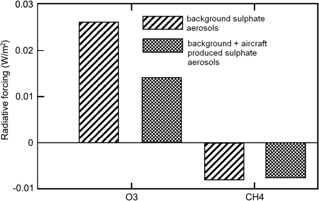
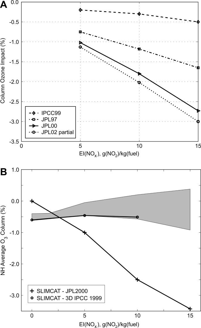
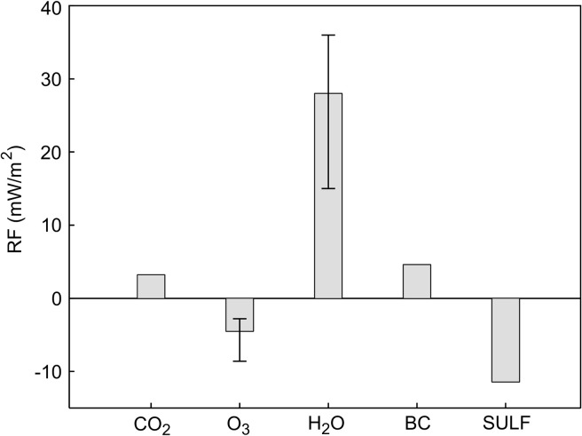
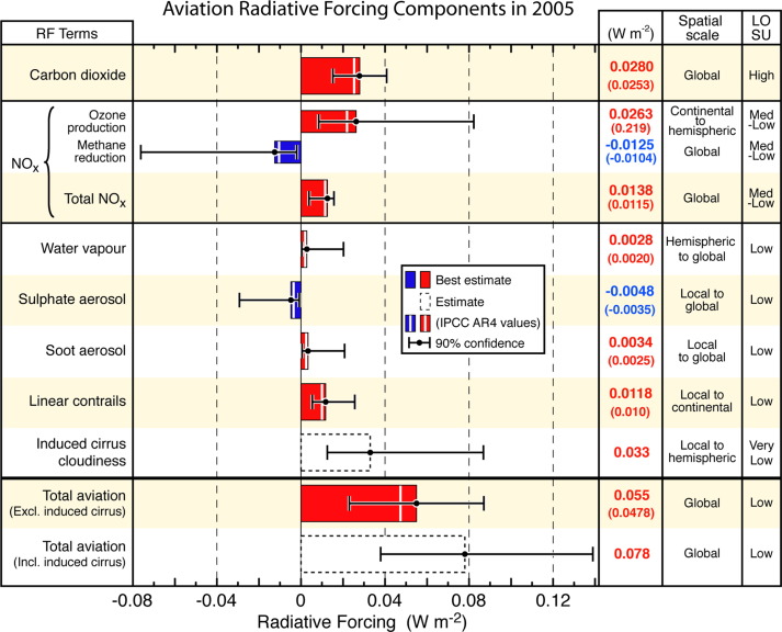
Aviation alters the composition of the atmosphere globally and can thus drive climate change and ozone depletion. The last major international assessment of these impacts was made by the Intergovernmental Panel on Climate Change (IPCC) in 1999. Here, a comprehensive updated assessment of aviation is provided. Scientific advances since the 1999 assessment have reduced key uncertainties, sharpening the quantitative evaluation, yet the basic conclusions remain the same. The climate impact of aviation is driven by long-term impacts from CO₂ emissions and shorter-term impacts from non-CO₂ emissions and effects, which include the emissions of water vapour, particles and nitrogen oxides (NO _x ). The present-day radiative forcing from aviation (2005) is estimated to be 55 mW m^-2 (excluding cirrus cloud enhancement), which represents some 3.5% (range 1.3-10%, 90% likelihood range) of current anthropogenic forcing, or 78 mW m^-2 including cirrus cloud enhancement, representing 4.9% of current forcing (range 2-14%, 90% likelihood range). According to two SRES-compatible scenarios, future forcings may increase by factors of 3-4 over 2000 levels, in 2050. The effects of aviation emissions of CO₂ on global mean surface temperature last for many hundreds of years (in common with other sources), whilst its non-CO₂ effects on temperature last for decades. Much progress has been made in the last ten years on characterizing emissions, although major uncertainties remain over the nature of particles. Emissions of NO _x result in production of ozone, a climate warming gas, and the reduction of ambient methane (a cooling effect) although the overall balance is warming, based upon current understanding. These NO _x emissions from current subsonic aviation do not appear to deplete stratospheric ozone. Despite the progress made on modelling aviation's impacts on tropospheric chemistry, there remains a significant spread in model results. The knowledge of aviation's impacts on cloudiness has also improved: a limited number of studies have demonstrated an increase in cirrus cloud attributable to aviation although the magnitude varies: however, these trend analyses may be impacted by satellite artefacts. The effect of aviation particles on clouds (with and without contrails) may give rise to either a positive forcing or a negative forcing: the modelling and the underlying processes are highly uncertain, although the overall effect of contrails and enhanced cloudiness is considered to be a positive forcing and could be substantial, compared with other effects. The debate over quantification of aviation impacts has also progressed towards studying potential mitigation and the technological and atmospheric tradeoffs. Current studies are still relatively immature and more work is required to determine optimal technological development paths, which is an aspect that atmospheric science has much to contribute. In terms of alternative fuels, liquid hydrogen represents a possibility and may reduce some of aviation's impacts on climate if the fuel is produced in a carbon-neutral way: such fuel is unlikely to be utilized until a 'hydrogen economy' develops. The introduction of biofuels as a means of reducing CO₂ impacts represents a future possibility. However, even over and above land-use concerns and greenhouse gas budget issues, aviation fuels require strict adherence to safety standards and thus require extra processing compared with biofuels destined for other sectors, where the uptake of such fuel may be more beneficial in the first instance.

Keywords: Aviation; Climate; Ozone depletion; Radiative forcing.

Fig. 1

Particle emission characteristics of the PartEmis combustor operated with medium fuel sulphur content, plotted in the context of emission characteristics measured for other aircraft engines at cruise conditions (adapted from Petzold et al., 2003; Copyright, 2003; American Geophysical Union. Modified by permission of American Geophysical Union).

Fig. 2

Number of soot particles and ice particles per kg of fuel in contrails versus fuel sulphur content (FSC), behind various aircraft: ATTAS (squares), B737 (circles), and A310 (diamonds). The full symbols with dashed lines approximate the mean soot particle emission indices measured for the three aircraft in non-contrail plumes. The grey symbols with error bars denote the number of ice particles formed per kg of fuel burned in contrails for the B737 and the ATTAS (Schumann et al., 2002, Schumann, 2005).

Fig. 3

Particle number emission index of detectable volatile particles in non-contrail plumes versus Fuel Sulphur Content (FSC) from various measurements, normalized to plume age 3 s, CNC cut-off 5 nm, and various sulphur conversion fractions ɛ and emission indices of condensable organic matter, EIOM (μg g⁻¹ fuel). The curves emphasizing the trend of observed particle number emission index with increasing FSC are results computed with a model (Kärcher et al., 2000) at the same values of plume age, cut-off, and EI of CIs of 2 × 10¹⁷ kg⁻¹, and different EIOM and ɛ values: 20 μg g⁻¹ fuel and 0.5% for dashed curve, and 30 μg g⁻¹ fuel and 8% for full curve (Schumann et al., 2002; Copyright, 2002; American Geophysical Union. Reproduced by permission of American Geophysical Union).

Fig. 4

Scheduled civil air traffic development from 1960 to 2007 in billions (10¹²) of revenue passenger kilometres (RPK) (source: ICAO traffic statistics from http://www.airlines.org/economics/traffic/World+Airline+Traffic.htm accessed, 19 Sept. 2007).

Fig. 5

Annual average growth rates in terms of revenue passenger kilometres (RPK) and long-term rolling average growth rate for scheduled civil aviation from 1970 to 2007 (source: ICAO traffic statistics from http://www.airlines.org/economics/traffic/World+Airline+Traffic.htm accessed, 19 Sept. 2007).

Fig. 6

Historical and present-day inventories, and future projections of civil aviation CO₂ emissions from a variety of sources: AERO2K (Eyers et al., 2005); ANCAT/EC2 (Gardner et al., 1998); CONSAVE (Berghof et al., 2005); FAST (Owen and Lee, 2006); IPCC (IPCC, 1999); NASA (Baughcum et al., 1996, Baughcum et al., 1998, Sutkus et al., 2001); SAGE (Kim et al., 2007). The open symbols indicate inventory analysis and the closed symbols indicate projections. Also shown are the CO₂ emissions implied by IEA fuel sales statistics (IEA, 2007). The IEA data represent the total of civil and military usage because all kerosene sales are included. The Sausen and Schumann (2000) data are also based on IEA. In the figure legend, the FAST, CONSAVE, and IPCC symbols are shown in an order that matches the scenario labels in the parentheses in each case (Lee et al., 2009).

Fig. 7

Supersonic aircraft fuel consumption (g m⁻² yr⁻¹) integrated over altitude (A) and (B) integrated over longitude.

Fig. 8

Zonal and annual mean lifetime of an H₂O perturbation calculated with climate-chemistry model E39/C-ATTILA (from Grewe and Stenke, 2008).

Fig. 9

Sketch of the main tropospheric O₃-related chemistry.

Fig. 10

Zonal and annual mean changes in (a) HO₂, (b) O₃ production, (c) O₃ loss, (d) NO_x, (e) net O₃ production, and (f) O₃ for 1991/92 air traffic emissions of 0.56 Tg N yr⁻¹. Regions are indicated where specific reactions occur, see text for details. Changes in production and loss rates are presented in a way that positive numbers indicate net O₃ production. Adapted from Grewe et al. (2002a).

Fig. 11

Taylor diagram for 4 models: TM3(T3), OsloCTM2 (C2), TOMCAT (TC), and LMDz/INCA(LZ) applied in the TRADEOFF project in a comparison of model output for various species with measurements made between 1995 and 1998 in an altitude range between 5.5 km and 13 km over the North Atlantic (adapted from Brunner et al., 2003).

Fig. 12

Frequency distributions of NO_x (pptv, left) and O₃ (ppbv, right) derived from NOXAR measurements (top) and E39/C model data (bottom). Data are analysed in a region of 50 hPa below the local tropopause. NOXAR consists of a year of measurements made on board regular passenger aircraft flying between Europe and Eastern USA and Europe and the Far East (adapted from Grewe et al., 2001).

Fig. 13

Globally integrated ozone response [DU] relative to aircraft NO_x emissions (Tg N yr⁻¹) for a number of model simulations (A) and, the ozone production efficiency (OPE, the number of ozone molecules produced per emitted NO_x molecule) (B). Data from the AEROCHEM2 project (Berntsen et al., 2003), the TRADEOFF project (Sausen et al., 2005, Stordal et al., 2006, Gauss et al., 2006), the QUANTIFY project (Hoor et al., 2009); E39/C model runs (Grewe et al., 2002b, Grewe, 2007), the GMI project (Rodriguez et al., 2003), OsloCTM2 runs (Isaksen et al., 2001, Gauss et al., 2006). Since individual tropospheric ozone lifetimes were not available, this was assumed to be 28 days for all models (see discussion in text).

Fig. 14

Sketch of the relationship between background tropospheric NO_x abundance and net ozone production, showing development at particular points in time.

Fig. 15

Time evolution of perturbations in ozone and methane total burden from a 1-month-pulse of aircraft NO_x emissions. Note that negative scale for ozone has been expanded for clarity (adapted from Stevenson et al., 2004.Copyright, 2004; American Geophysical Union. Modified by permission of American Geophysical Union).

Fig. 16

Impact of the location of an emission on the RF of O₃ (panel A) and CH₄ (panel B) in mW m⁻²; the negative ratio of both is shown in (panel C). The RF values at a certain pressure level and latitude refer to a sustained emission of 1 Tg N yr⁻¹ at that location.

Fig. 17

Annual globally averaged radiative forcing of O₃ and CH₄ (W m⁻²) for simulations with heterogeneous chemistry on background sulphate aerosols and simulations with heterogeneous chemistry on background plus aircraft produced sulphate aerosols (adapted from Pitari et al., 2002b; Copyright, 2004; American Geophysical Union. Modified by permission of American Geophysical Union).

Fig. 18

SLIMCAT modelled background zonal mean N₂O (ppbv) at an altitude of 32 km as a function of meteorological year (A) and zonal mean NO_y differences (ppbv) (B) at an altitude of 32 km. Differences are calculated between the integration with both subsonic and supersonic aircraft and the integration with only subsonic aircraft, as a function of meteorological year (adapted from Rogers et al., 2000).

Fig. 19

Northern Hemisphere total ozone column change as a function of EINO_x in 2015 for a supersonic fleet of 500 HSCTs (A) (adapted from Baughcum et al., 2003). Northern Hemisphere total ozone column change as a function of EINO_x in 2015 for a supersonic fleet of 500 HSCTs (B). The shaded area represents the range of model variability in IPCC (1999) (adapted from IPCC, 1999). The black line with symbol “+” represents the SLIMCAT model calculation with updated reaction rates (B) (adapted from Dessens et al., 2007).

Fig. 20

Frequency of the occurrence of type 1a PSCs (left), type 1b PSCs (middle) and type 2 PSCs (right) at model level 5 (approx. 475 K potential temperature) in the ‘no aircraft’ emission scenario (hatched curves) and the ‘supersonic’ scenario (thick curves) using the University of Oslo aircraft induced perturbations in H₂O and HNO₃ concentrations (Larsen et al., 2002).

Fig. 21

Summary of radiative forcing per component in 2050 (mW m⁻²), O₃ and H₂O radiative forcing average values and variability were calculated using the DLR model radiative code applied to O₃ and H₂O changes (S6-S4) calculated by UCAM, ULAQ, DLR and UiO CTMs (Pitari et al., 2008).

Fig. 22

Monthly changes in surface erythemal irradiance (percentage) for different emission scenarios defined in SCENIC (see Table 4) relative to the base scenario.

Fig. 23

Changes in global mean surface temperature for the year 2100 (solid bars) and for O₃ (dashed bars) for constant revenue passenger kilometres (RPK) of the total fleet (blue) and constant HSCT RPK (red). The product of both factors is added (green) for constant HSCT RPK. For each bar an uncertainty range is given, which represents minimum and maximum values. No bars are added when only one model has calculated chemical perturbations. In those cases the same uncertainty range has been assumed as for P4 for the calculation of the uncertainty of the product (Grewe et al., 2007).

Fig. 24

Distribution of relative humidity over ice (RHI) outside of (left panel) and inside (right panel) cirrus clouds measured during the INCA project campaign in Punta Arenas (Southern Hemisphere – SH) and Prestwick (Northern Hemisphere – NH). The distributions are normalized with the number of data points in the respective 100% bin and all RHI values were binned into 4% intervals. The precision of RHI measurements is ±3% (1σ-limits), with horizontal bars depicting the 3σ-limits. The colored arrows mark the cut-offs derived from the modelled distributions (homogeneous – red; heterogeneous – blue; mixed homo-/heterogeneous for concentrations of total ice nuclei 0.1 cm⁻³ – black; mixed homo-/heterogeneous for concentrations of total ice nuclei 0.001 cm⁻³ – green) (Haag et al. (2003).

Fig. 25

In-cloud ice crystal number concentration (cm⁻³) (N_i) calculated with the Kärcher et al. (2006) (KL, left) and with the Liu and Penner (2005) (LP, right) ice nucleation parameterization at 140 hPa (lower) and 190 hPa (upper). Aerosol and meteorological fields are from the coupled IMPACT-CAM3 model run.

Fig. 26

Four month (January, April, July, October) average TOA net forcing (W m⁻²) from all anthropogenic aerosols (A), aircraft generated soot (B), anthropogenic soot from surface sources (C) and anthropogenic sulphate (D). The Kärcher et al. (2006) parameterization together with the 3-mode sulfate aerosol model is used to calculate ice nucleation (adapted from Penner et al., 2009).

Fig. 27

Response of RF (W m⁻²) and T (°K ) to aviation emissions. (A &B) decay timescales of RF and T from different components following cessation of emissions in 2000. (C) An aviation fleet ‘pulse’ response of T assuming instantaneous fuel burn of 100 Tg C yr⁻¹ and EINO_x of 12 (from model of Lim et al. (2007), tuned to Stevenson et al. (2004)).

Fig. 28

Radiative forcing components from global aviation as evaluated from preindustrial times until 2005. Bars represent updated best estimates or an estimate in the case of aircraft-induced cirrus cloudiness (AIC). IPCC AR4 values are indicated by the white lines in the bars as reported by Forster et al. (2007a). The induced cloudiness (AIC) estimate includes linear contrails. Numerical values are given on the right for both IPCC AR4 (in parentheses) and updated values. Error bars represent the 90% likelihood range for each estimate. The median value of total radiative forcing from aviation is shown with and without AIC. The median values and uncertainties for the total NO_x RF and the two total aviation RFs are calculated using a Monte Carlo simulation. The Total NO_x RF is the combination of the CH₄ and O₃ RF terms, which are also shown here. The AR4 value noted for the Total NO_x term is the sum of the AR4 CH₄ and O₃ best estimates. Note that the confidence interval for ‘Total NO_x’ is due to the assumption that the RFs from O₃ and CH₄ are 100% correlated; however, in reality, the correlation is likely to be less than 100% but to an unknown degree (see text). The geographic spatial scale of the radiative forcing from each component and the level of scientific understanding (LOSU) are also shown on the right (Lee et al., 2009).

Fig. 29

Charactericstic NO_x of in-service engines according to CAEP NO_x regulatory parameter, Dp/foo (g NO_x/kN thrust at static sea-level test conditions) vs overall pressure ratio of engine. The CAEP medium term (MT) and long term (LT) technology goals are shown as lines.

Fig. 30

Altitude distribution of ice supersaturated layers over Lindenberg, Germany, taken from corrected radiosonde humidity measurements (cf. Spichtinger et al., 2003) (A). A change in flight levels of at least ± 2 km would be needed to avoid half of the ice supersaturation. Probability of being in an ice supersaturated layer after an altitude change from the centre level of the ice-supersaturated region (B). A flight level change of ±300 m suffices to avoid ice-supersaturation on a case by case basis (analysis K. Gierens and U. Schumann).

References

1. ACARE . 2001. European Aeronautics: a Vision for 2020. Meeting Society's Needs and Winning Global Leadership.http://www.acare4europe.org/docs/Vision%202020.pdf Report of the group of personalities. (accessed 30.05.09)
1. Anderson B.E., Chen G., Blake D.R. Hydrocarbon emissions from a modern commercial airliner. Atmos. Environ. 2006;40:3601–3612.
1. Anonymous . Aeronautics Science and Technology Subcommittee, Committee on Technology, National Science and Technology Council; US: 2007. National Plan for Aeronautics Research and Devlopment and Related Infrastructure.http://www.ostp.gov/aeroplans/pdf/aero_rd_plan_final_21_dec_2007.pdf (accessed 30.05.09)
1. Appleman H. The formation of exhaust contrails by jet aircraft. Bull. Amer. Meteor. Soc. 1953;34:14–20.
1. Archuleta C.M., DeMott P.J., Kreidenweis S.M. Ice nucleation by surrogates for atmospheric mineral dust and mineral dust/sulfate particles at cirrus temperatures. Atmos. Chem. Phys. 2005;5:2617–2634.