A gravity-based three-dimensional compass in the mouse brain

Abstract

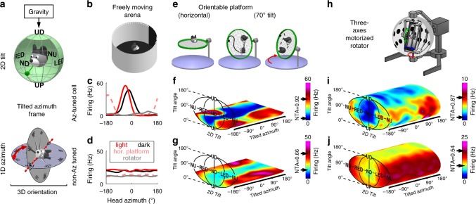
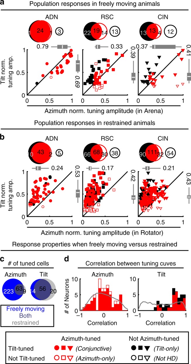
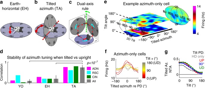
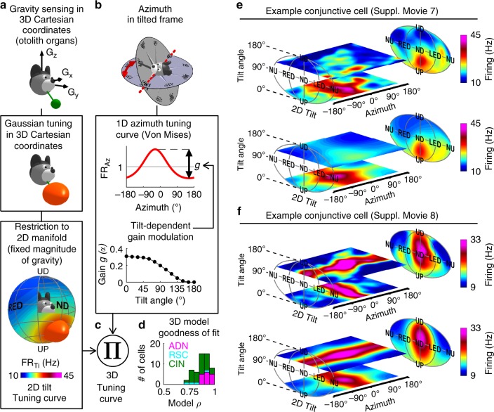
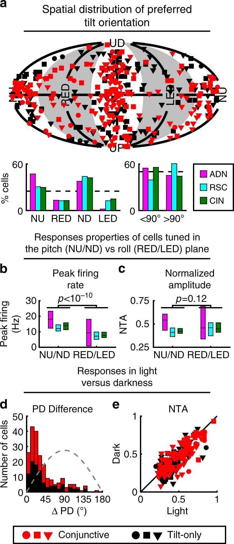
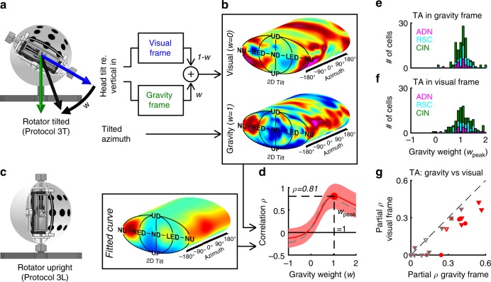
Gravity sensing provides a robust verticality signal for three-dimensional navigation. Head direction cells in the mammalian limbic system implement an allocentric neuronal compass. Here we show that head-direction cells in the rodent thalamus, retrosplenial cortex and cingulum fiber bundle are tuned to conjunctive combinations of azimuth and tilt, i.e. pitch or roll. Pitch and roll orientation tuning is anchored to gravity and independent of visual landmarks. When the head tilts, azimuth tuning is affixed to the head-horizontal plane, but also uses gravity to remain anchored to the allocentric bearings in the earth-horizontal plane. Collectively, these results demonstrate that a three-dimensional, gravity-based, neural compass is likely a ubiquitous property of mammalian species, including ground-dwelling animals.

Fig. 1. Three-dimensional response of two example cells.

a Proposed framework for 3D orientation. Top: tilt is measured by sensing the gravity vector (green pendulum) in egocentric coordinates, resulting in a 2D spherical topology. Bottom: azimuth has a circular topology, and is measured by rotating an earth-horizontal compass in alignment with the head-horizontal plane (TA frame). b Schematic of the arena used to identify azimuth-tuned cells in the horizontal plane. c, d Example azimuth tuning of a traditional HD cell, i.e. tuned to azimuth (Az-tuned) in the ADN (c) and another cell not tuned to azimuth (non-Az-tuned cell) in the cingulum (d), as the mouse walks freely in light (red) and darkness (black) in a horizontal arena (shown in b), on a platform oriented horizontally (shown in e, left; broken pink lines) and in the rotator (shown in h; gray lines). The azimuth-tuned cell showed significant tuning with different preferred directions (PD) in all setups, although response was strongly attenuated in the rotator (compare gray with red/pink lines). e Schematic of a 3D orientable platform used to measure 3D tuning. f, g Tuning curves for the two cells in c and d, obtained from responses as the mouse foraged on the orientable platform (shown in e). Firing rate is shown as a heat map in 3D space (Supplementary Movies 1, 2). The peak and trough of the average tilt response (across all azimuths) are indicated with arrows on the color scale; NTA = (peak-trough)/peak. Note that tuning curves are restricted to 60° tilt (Methods). h Schematic of a rotator used to measure full 3D tuning curves. i, j Tuning curves for the two cells in c, f and d, g as the mouse was passively re-oriented uniformly throughout the full 3D space using the rotator (Supplementary Movies 3–5).

Fig. 2. Population azimuth and tilt tuning in freely moving vs. restrained animals.

a Summary of tuning prevalence during unrestrained motion. Azimuth tuning was derived from data in the freely moving arena (Fig. 1b). Tilt tuning was derived from data on the 3D platform (Fig. 1e). For each panel, Venn diagrams (top) indicate the number of tilt-tuned (filled black discs) and azimuth-tuned (red discs) cells. Conjunctive cells appear at the intersection of these discs. Open discs illustrate cells responsive to neither tilt nor azimuth. The scatterplots (bottom) indicate the normalized modulation amplitude of responsive cells. The boxes and whiskers represent the median (white line), 95% confidence interval (boxes) and upper/lower quartiles (whiskers) of the azimuth modulation of azimuth-tuned cells (top) and tilt modulation of tilt-tuned cells (right). Different symbols (based on recorded area) are color-coded based on cell type (Conjunctive: filled red; Azimuth-only: open red; Tilt-only: filled black). b Prevalence of tilt tuning in the rotator (Fig. 1h) and azimuth tuning (when moving freely). Format as in a. c Comparison of responsiveness for cells tested in both restrained and freely foraging animals. Venn diagrams with the number of cells tuned when moving freely (blue) in the arena (azimuth tuning) or 3D platform (tilt tuning) and restrained in the rotator (gray). Cells tuned under both conditions appear at the intersection of both discs. d Pixel-by-pixel correlation of the fitted azimuth (left) and tilt (right) tuning curves (only cells tuned under both freely moving and restrained conditions are included). For tilt tuning, the rotator data were re-analyzed by restricting tilt angles up to 60° (to match the conditions in the platform). Gray: expected distribution if tuning curves shift randomly (H0), computed by randomly shuffling the cells. Source data are provided as a Source Data file.

Fig. 3. Encoding of azimuth is also influenced by gravity.

a Illustration of the earth-horizontal (EH) frame, where azimuth direction is projected onto the earth-horizontal plane (dashed red line). b Tilted azimuth (TA) frame, where azimuth is defined by rotating head direction (gray vector) towards the horizontal plane instead of projecting it. The head has the same 3D orientation in a and b but its azimuth is different in the two frames (EH: 165°; TA: 135°). c Dual-axis rule for updating TA, illustrated by an example trajectory (red) where the animal travels in 3D across three orthogonal surfaces (numbered 1 to 3). Head azimuth is updated when the head rotates in yaw within one surface (first rule, cyan arrows) or in the earth-horizontal plane (second rule, green arrow when transitioning from surface 2 to 3). The first rule tracks azimuth and the second rule ensures that the brain compass always matches the EH compass along the line intersecting the two planes (the 0–180° line in b). d Correlation between azimuth tuning curves when upright (<45° tilt) vs. tilted (>60°) in YO, EH and TA frames. Colored bars: Median correlation in each brain region. Lines: 95% confidence intervals. Gray bars: data pooled across all cells. p-value based on a Wilcoxon-signed rank test across all cells. e 3D tuning curve of an example azimuth-only cell, showing horizontal slices at tilt angles of 30° and 110° (see animations in Supplementary Movie 7). The average tilt tuning (across all azimuths) is shown on the right panel. f Average azimuth tuning curve of all azimuth-only cells that maintained their azimuth tuning in the rotator (n = 10), averaged across all tilt orientations (γ), computed at tilt angles (α) ranging from 0 to 180° and centered on PD = 0°. g Average normalized tuning amplitude of the azimuth tuning curve as a function of tilt angle, computed for azimuth-only cells (n = 10, gray) and conjunctive cells with preferred tilt directions near upright (<75° tilt, red, n = 16), near 90° tilt (±15°, blue, n = 22) and near upside-down (>105°, green, n = 15). Source data are provided as a Source Data file.

Fig. 4. Modeling 3D responses.

a Modeling tilt tuning. Top: Gravity is a 3D vector (green) sensed in egocentric Cartesian coordinates by the otolith organs. Middle: to model tilt tuning, we first assume a 3D Gaussian function (orange ellipsoid) in this Cartesian space. Bottom: on earth, the magnitude of gravity is constant. Therefore, we restrict the tilt tuning curve to a 2D sphere surrounding the head, which corresponds to the egocentric gravity vector experienced when tilting on earth. b Modeling azimuth tuning. Azimuth is expressed in a TA frame (top), and tuning is modeled as a von Mises distribution combined with a tilt-dependent gain factor (Fig. 3g). c 3D tuning defined by the product of these two curves. d Distribution of the model’s coefficient of correlation (ρ) across areas. e, f Experimentally measured 3D tuning curves (top) from two conjunctive cells that maintain their azimuth tuning in the rotator and fitted tuning curves (bottom), represented as color maps in 3D space (animated in Supplementary Movies 8, 9). The cell is e is the same as in a, b. Source data are provided as a Source Data file.

Fig. 5. Summary of 3D tilt tuning (based on full tuning curves measured in the rotator).

a Top: Distribution of tilt PDs. Red: Conjunctive (azimuth and tilt) cells; Black: tilt-only cells. Circles, squares, triangles: ADN, RSC, CIN, respectively. Bottom: Number of cells with PD in the roll (RED/LED) or pitch (ND/NU) plane; and in upper (<90° tilt) or lower (>90° tilt) hemisphere, color-coded separately for each area (AND, CIN, RSC). b, c Comparison of peak firing rate (b) and NTA (c) of the tilt tuning curves of neurons with PD in the roll and pitch plane, color-coded by regions. Boxes represent the median and 95% confidence interval of the median. p-values are based on a Wilcoxon-rank sum test. d Distributions of absolute difference in tilt PD for light vs. darkness for conjunctive (red) and tilt-only (black) cells. Gray dashed line: expected distribution if PDs are independently distributed on a sphere. e Comparison of tilt peak-to-trough normalized tuning amplitude computed from Gaussian fits (Methods) in darkness vs. light. Red: Conjunctive (azimuth and tilt) cells; Black: tilt-only cells. Source data are provided as a Source Data file.

Fig. 6. Tilt tuning is anchored to gravity.

a, b Rationale of the analysis and 3D tuning curve of an example cell when tilt is expressed relative to visually referenced vertical (b, upper tuning curve) or gravitational vertical (b, lower tuning curve). c Reference curve computed with the rotator upright. d Red: Coefficient of correlation between the tuning curves in a and the reference in b, as a function of the weight w, assuming TA is referenced to gravity. The red band indicates 95% confidence interval. Broken gray line: same correlation, computed assuming that TA is anchored to vision. e, f Gravity weight at which the correlation is maximal for all tilt-tuned cells where w_peak is significantly higher than 0, computed when TA is referenced to gravity (e) or vision (f). g Comparison of the partial correlation (with the effect of gravity removed) of azimuth-tuned cells, assuming that TA is anchored to a gravity or visually referenced frame. Open/filled symbols: azimuth-only and conjunctive cells. Red/gray: cells where the difference between the two frames is significant or not. Source data are provided as a Source Data file.

References

1. Webber DM, Aitken JP, O’Dor RK. Costs of locomotion and vertic dynamics of cephalopods and fish. Physiol. Biochem. Zool. 2000;73:651–662. doi: 10.1086/318100. - DOI - PubMed
1. Gaveau J, Berret B, Angelaki DE, Papaxanthis C. Direction-dependent arm kinematics reveal optimal integration of gravity cues. Elife. 2016;5:e16394. doi: 10.7554/eLife.16394. - DOI - PMC - PubMed
1. McIntyre J, Zago M, Berthoz A, Lacquaniti F. Does the brain model Newton’s laws? Nat. Neurosci. 2001;4:693–694. doi: 10.1038/89477. - DOI - PubMed
1. Sack FD. Plant gravity sensing. Int. Rev. Cytol. 1991;127:193–252. doi: 10.1016/S0074-7696(08)60695-6. - DOI - PubMed
1. Bender JA, Frye MA. Invertebrate solutions for sensing gravity. Curr. Biol. 2009;19:R186–R190. doi: 10.1016/j.cub.2008.12.024. - DOI - PubMed
Publication types