Circular inference in bistable perception

Abstract

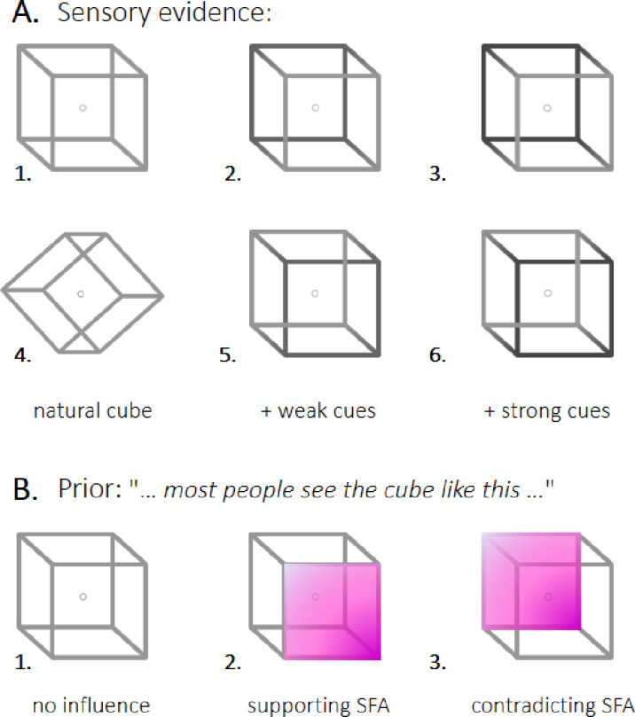
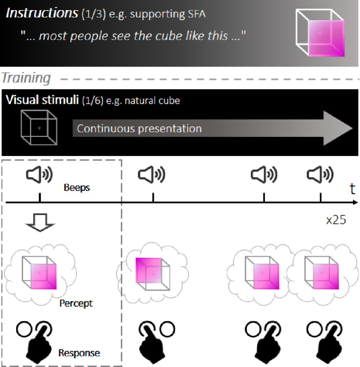
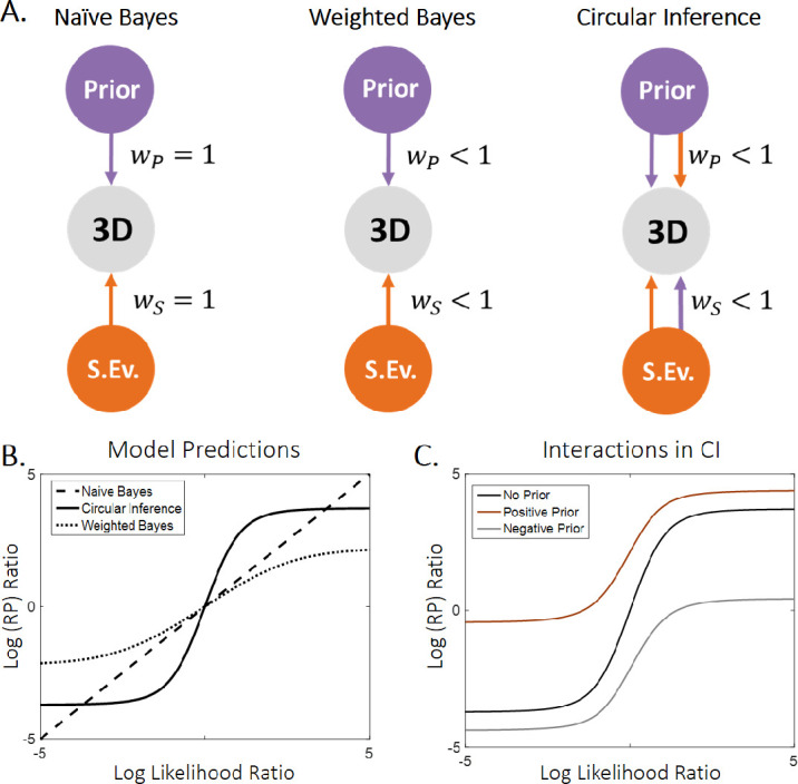
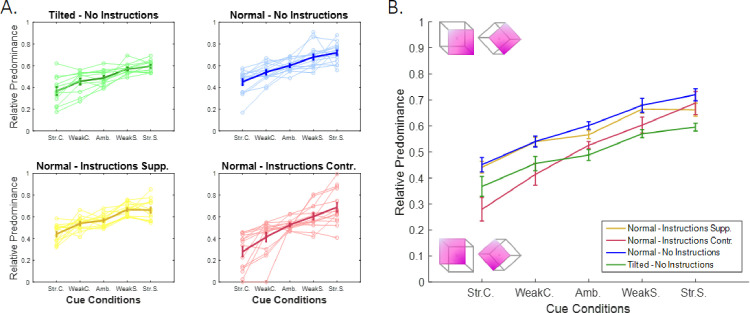
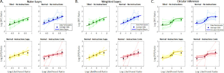
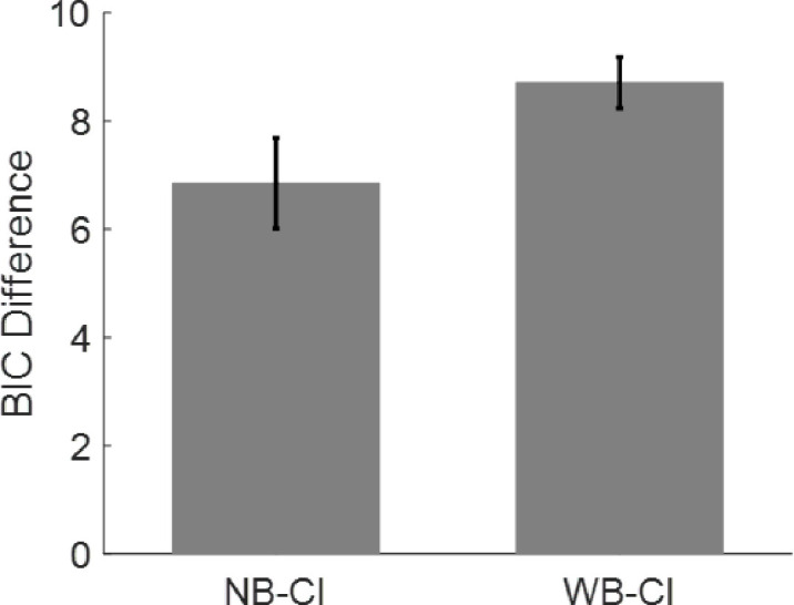
When facing ambiguous images, the brain switches between mutually exclusive interpretations, a phenomenon known as bistable perception. Despite years of research, a consensus on whether bistability is driven primarily by bottom-up or top-down mechanisms has not been achieved. Here, we adopted a Bayesian approach to reconcile these two theories. Fifty-five healthy participants were exposed to an adaptation of the Necker cube paradigm, in which we manipulated sensory evidence and prior knowledge. Manipulations of both sensory evidence and priors significantly affected the way participants perceived the Necker cube. However, we observed an interaction between the effect of the cue and the effect of the instructions, a finding that is incompatible with Bayes-optimal integration. In contrast, the data were well predicted by a circular inference model. In this model, ambiguous sensory evidence is systematically biased in the direction of current expectations, ultimately resulting in a bistable percept.

Figure 1.

Stimuli and instructions. (A) Different Necker cubes were used to induce bistable perception, in which the 2D figure is perceived as a 3D cube with either the left or the right side located closer to the observer. Even in the case of the completely ambiguous stimulus (1), people have an implicit preference to interpret the cube as seen from above (SFA interpretation), which was interpreted as an implicit prior. This prior was refuted by tilting the stimulus (4). Sensory evidence was manipulated by adding visual cues in the form of contrasts (2-3 and 5-6). The contrast was strong (3 and 6) or weak (2 and 5) and supported (2 and 3) or contradicted (5 and 6) the implicit prior. (B) A further manipulation of the prior was achieved by providing correct or wrong information to the participants about which interpretation was generally stronger (explicit prior). The instructions either supported or contradicted the implicit prior. An additional control group received no particular instructions. Crucially, all groups received the same visual instructions (including the stimulus and the two possible interpretations) and the differences were only the verbal instructions to avoid additional priming effects. Note that the color used in the present figure has only been added for illustration purposes; during the experiment, participants were presented with full cubes.

Figure 2.

Experimental design. The task was inspired by a previous study (Mamassian & Goutcher, 2005). Instructions were provided at the beginning of the experiment (each participant received one set of instructions, creating a between-subjects design) and were followed by a short training phase to familiarize participants with the stimulus and the switches. During each run, one version of the cube was continuously presented to the participants, who were asked to discontinuously report their dominant percept by pressing a button every time a sound was heard. Each run consisted of 25 sound trials (mean inter-sound interval = 1.5 seconds). The main experiment consisted of 30 runs separated into six blocks of five runs each. In each block, a different variant of the stimulus was used. The first and fourth blocks always contained the ambiguous cube. The four cue conditions were randomly assigned to the four remaining blocks.

Figure 3.

Models and model predictions. (A) Three different models were used to fit the data. The simplest model (naïve Bayes [NB], left panel) consisted of a simple addition of the sensory evidence and prior on the log scale and is equivalent to a three-layer generative model in which all the connections are equal to 1. The weighted Bayes (WB) model (middle panel) further assumes that only partial trust exists between the nodes of the generative model. Importantly, both the NB and WB models do exact inference. Finally, we used a circular inference (CI) model (right panel) that further allows reverberation and overcounting of sensory evidence and prior knowledge. (B) The log(RP) ratio predicted by the models as a function of the log-likelihood ratio. The NB model predicts a linear dependence, whereas both the WB and CI models predict sigmoid curves (due to the saturation imposed by the weights). Furthermore, the three models generate different predictions about the slope of the curves around zero. The NB and WB models predict a slope of 1 and less than 1, respectively, and only the CI model predicts a slope greater than 1. (C) In the CI model, the slope of the log-likelihood/log-posterior curve also depends on the log-prior as a result of the reverberations, indicating an interaction between the two different types of information (Leptourgos et al., 2017). Weaker priors are associated with steeper sigmoid curves. The reason is the saturating effect of the weight when priors and sensory inputs are congruent (they are both positive/negative).

Figure 4.

Relative predominance between conditions. (A) The four subplots illustrate the four different prior conditions: tilted cube (top left plot, green; n = 12) or normal cube with no instructions (top right plot, blue; n = 15), supporting instructions (bottom left plot, yellow; n = 14) or contradictory instructions (bottom right plot, red; n = 14). The x-axis presents the five cue conditions, ranging from a strong cue supporting the SFB interpretation (left panels) to a strong cue supporting the SFA interpretation (right panels). Thin lines correspond to the behaviors of single participants (outliers are not presented), and thick lines represent the average RP for each group calculated after removing the outliers (±  SE). (B) Between-groups comparison of average RP values. A linear mixed-effects model revealed significant effects of sensory evidence (p < 0.001) and the prior (contradictory instructions, p < 0.001) and tilt (p < 0.001) manipulations. We also observed a cue x instruction interaction for the contradictory instructions (red curve) compared with supporting instructions (yellow curve, p = 0.016) and the tilted cube (green curve, p = 0.021).

Figure 5.

Observed and predicted log(RP) ratios as a function of the log-likelihood ratio. Different colors correspond to different prior conditions. Thin lines represent data from single participants, highlighted points correspond to average RPs (± SE), and thick lines illustrate the predictions generated by the models. The three models are presented separately, since the likelihood was itself considered a free parameter [(A): NB, (B): WB, and (C): CI]. The models were fitted to aggregated data from all participants by minimizing the mean squared distance between the observed and predicted log(RP) ratios.

Figure 6.

Comparison of the three models. The CI model outperforms both the NB and WB models (note that a positive difference indicates lower BIC score for CI and thus better performance). Fitting was repeated multiple times, and one of the participants was removed each time (“Jackknife” resampling method). In all cases, (55 possible subsamples), the CI model outperformed the other two models by producing a difference in BIC scores greater than 4.5, whereas in 48/55 cases, the difference was greater than 6. Error bars correspond to standard deviations of the jackknife estimates.

References

1. Acerbi L., Vijayakumar S., & Wolpert D. M. (2014). On the origins of suboptimality in human probabilistic inference. PLoS Computational Biology, 10(6), 1–23, 10.1371/journal.pcbi.1003661. - DOI - PMC - PubMed
1. Babich S., & Standing L. (1981). Satiation effects with reversible figures. Perceptual and Motor Skills, 52, 203–210, 10.2466/pms.1981.52.1.203. - DOI - PubMed
1. Baker D. H., & Graf E. W. (2009). Natural images dominate in binocular rivalry. Proceedings of the National Academy of Sciences, 106(13), 5436–5441, 10.1073/pnas.0812860106. - DOI - PMC - PubMed
1. Beck J. M., Ma W. J., Pitkow X., Latham P. E., & Pouget A. (2012). Not noisy, just wrong: the role of suboptimal inference in behavioral variability. Neuron, 74(1), 30–39, 10.1016/j.neuron.2012.03.016. - DOI - PMC - PubMed
1. Bishop C. (2006). Pattern Recognition and Machine Learning. Berlin: Springer.
Publication types